Chapter 4. Predicting Forest Cover with Decision Trees
Prediction is very difficult, especially if itâs about the future.
Niels Bohr
In the late nineteenth century, the English scientist Sir Francis Galton was busy measuring things like peas and people. He found that large peas (and people) had larger-than-average offspring. This isnât surprising. However, the offspring were, on average, smaller than their parents. In terms of people: the child of a seven-foot-tall basketball player is likely to be taller than the global average but still more likely than not to be less than seven feet tall.
As almost a side effect of his study, Galton plotted child versus parent size and noticed there was a roughly linear relationship between the two. Large parent peas had large children, but slightly smaller than themselves; small parents had small children, but generally a bit larger than themselves. The lineâs slope was therefore positive but less than 1, and Galton described this phenomenon as we do today, as regression to the mean.
Although maybe not perceived this way at the time, this line was, to me, an early example of a predictive model. The line links the two values, and implies that the value of one suggests a lot about the value of the other. Given the size of a new pea, this relationship could lead to a more accurate estimate of its offspringâs size than simply assuming the offspring would be like the parent or like every other pea.
Fast Forward to Regression
More than a century of statistics later, and since the advent of modern machine learning and data science, we still talk about the idea of predicting a value from other values as regression, even though it has nothing to do with slipping back toward a mean value, or indeed moving backward at all. Regression techniques also relate to classification techniques. Generally, regression refers to predicting a numeric quantity like size or income or temperature, whereas classification refers to predicting a label or category, like âspamâ or âpicture of a cat.â
The common thread linking regression and classification is that both involve predicting one (or more) values given one (or more) other values. To do so, both require a body of inputs and outputs to learn from. They need to be fed both questions and known answers. For this reason, they are known as types of supervised learning.
Classification and regression are the oldest and most well-studied types of predictive analytics. Most algorithms you will likely encounter in analytics packages and libraries are classification or regression techniques, like support vector machines, logistic regression, naïve Bayes, neural networks, and deep learning. Recommenders, the topic of Chapter 3, were comparatively more intuitive to introduce, but are also just a relatively recent and separate subtopic within machine learning.
This chapter will focus on a popular and flexible type of algorithm for both classification and regression: decision trees, and the algorithmâs extension, random decision forests. The exciting thing about these algorithms is that, with all due respect to Mr. Bohr, they can help predict the futureâor at least, predict the things we donât yet know for sure, like the likelihood you will buy a car based on your online behavior, whether an email is spam given its words, or which acres of land are likely to grow the most crops given their location and soil chemistry.
Vectors and Features
To explain the choice of the data set and algorithm featured in this chapter, and to begin to explain how regression and classification operate, it is necessary to briefly define the terms that describe their input and output.
Consider predicting tomorrowâs high temperature given todayâs weather. There is nothing wrong with this idea, but âtodayâs weatherâ is a casual concept that requires structuring before it can be fed into a learning algorithm.
Really, it is certain features of todayâs weather that may predict tomorrowâs temperature, such as:
-
Todayâs high temperature
-
Todayâs low temperature
-
Todayâs average humidity
-
Whether itâs cloudy, rainy, or clear today
-
The number of weather forecasters predicting a cold snap tomorrow
These features are also sometimes called dimensions, predictors, or just variables. Each of these features can be quantified. For example, high and low temperatures are measured in degrees Celsius, humidity can be measured as a fraction between 0 and 1, and weather type can be labeled cloudy, rainy, or clear. The number of forecasters is, of course, an integer count. Todayâs weather might therefore be reduced to a list of values like 13.1,19.0,0.73,cloudy,1.
These five features together, in order, are known as a feature vector, and can describe any dayâs weather. This usage bears some resemblance to use of the term vector in linear algebra, except that a vector in this sense can conceptually contain nonnumeric values, and even lack some values.
These features are not all of the same type. The first two features are measured in degrees Celsius, but the third is unitless, a fraction. The fourth is not a number at all, and the fifth is a number that is always a nonnegative integer.
For purposes of discussion, this book will talk about features in two
broad groups only: categorical features and numeric features. In this context, numeric features are those that can be quantified by a number and have a meaningful ordering. For example, itâs meaningful to say that todayâs high was 23ºC, and that this is higher than yesterdayâs high of 22ºC. All of the features mentioned previously are numeric, except the weather type. Terms like clear are not numbers, and have no ordering. It is meaningless to say that cloudy is larger than clear. This is a categorical feature, which instead takes on one of several discrete values.
Training Examples
A learning algorithm needs to train on data in order to make predictions. It requires a large number of inputs, and known correct outputs, from historical data. For example, in this problem, the learning algorithm would be given that, one day, the weather was between 12º and 16ºC, with 10% humidity, clear, with no forecast of a cold snap; and the following day, the high temperature was 17.2ºC. With enough of these examples, a learning algorithm might learn to predict the following dayâs high temperature with some accuracy.
Feature vectors provide an organized way to describe input to a learning algorithm (here: 12.5,15.5,0.10,clear,0). The output, or target, of the prediction can also be thought of as a feature. Here, it is a numeric feature: 17.2. Itâs not uncommon to simply include the target as another feature in the feature vector. The entire training example might be thought of as 12.5,15.5,0.10,clear,0,17.2. The collection of all of these examples is known as the training set.
Note that regression problems are just those where the target is a numeric feature, and classification problems are those where the target is categorical. Not every regression or classification algorithm can handle categorical features or categorical targets; some are limited to numeric features.
Decision Trees and Forests
It turns out that the family of algorithms known as decision trees can naturally handle both categorical and numeric features. Building a single tree can be done in parallel, and many trees can be built in parallel at once. They are robust to outliers in the data, meaning that a few extreme and possibly erroneous data points might not affect predictions at all. They can consume data of different types and on different scales without the need for preprocessing or normalization, which is an issue that will reappear in Chapter 5.
Decision trees generalize into a more powerful algorithm, called random decision forests.
Their flexibility makes these algorithms worthwhile to examine in this chapter, where Spark
MLlibâs DecisionTree and RandomForest implementation will be applied to a data set.
Decision treeâbased algorithms have the further advantage of being comparatively
intuitive to understand and reason about. In fact, we all probably use the same reasoning
embodied in decision trees, implicitly, in everyday life. For example, I sit down to have
morning coffee with milk. Before I commit to that milk and add it to my brew,
I want to predict: is the milk spoiled? I donât know for sure.
I might check if the use-by date has passed. If not, I predict no, itâs not spoiled.
If the date has passed, but that was three or fewer days ago, I take my chances and predict no, itâs not spoiled.
Otherwise, I sniff the milk. If it smells funny, I predict yes, and
otherwise no.
This series of yes/no decisions that lead to a prediction are what decision trees embody. Each decision leads to one of two results, which is either a prediction or another decision, as shown in Figure 4-1. In this sense, it is natural to think of the process as a tree of decisions, where each internal node in the tree is a decision, and each leaf node is a final answer.
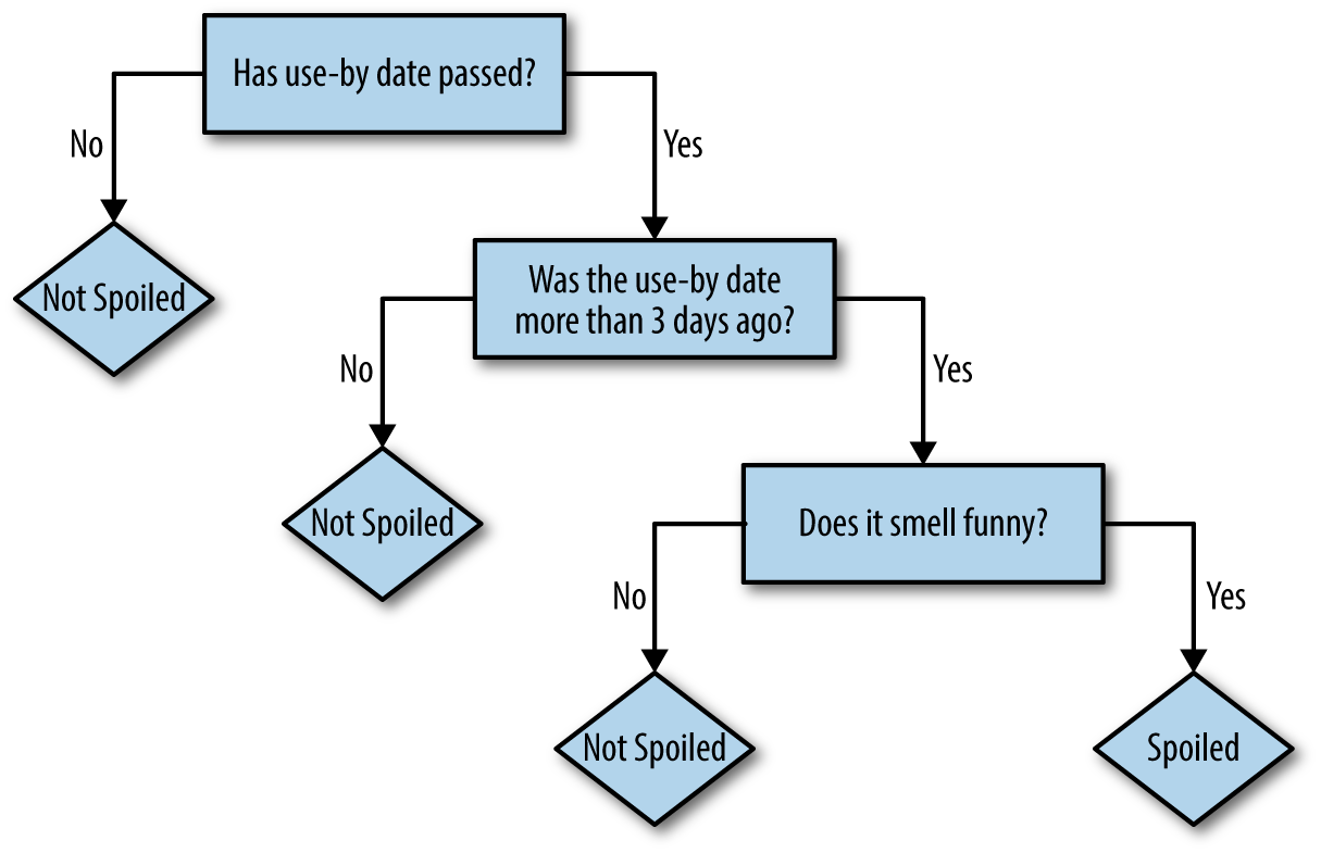
Figure 4-1. Decision tree: is it spoiled?
The preceding rules were ones I learned to apply intuitively over years of bachelor lifeâthey seemed like rules that were both simple and also usefully differentiated cases of spoiled and nonspoiled milk. These are also properties of a good decision tree.
That is a simplistic decision tree, and was not built with any rigor. To elaborate, consider another example. A robot has taken a job in an exotic pet store. It wants to learn, before the shop opens, which animals in the shop would make a good pet for a child. The owner lists nine pets that would and wouldnât be suitable before hurrying off. The robot compiles the information found in Table 4-1 from examining the animals.
| Name | Weight (kg) | # Legs | Color | Good pet? |
|---|---|---|---|---|
Fido |
20.5 |
4 |
Brown |
Yes |
Mr. Slither |
3.1 |
0 |
Green |
No |
Nemo |
0.2 |
0 |
Tan |
Yes |
Dumbo |
1390.8 |
4 |
Gray |
No |
Kitty |
12.1 |
4 |
Gray |
Yes |
Jim |
150.9 |
2 |
Tan |
No |
Millie |
0.1 |
100 |
Brown |
No |
McPigeon |
1.0 |
2 |
Gray |
No |
Spot |
10.0 |
4 |
Brown |
Yes |
Although a name is given, it will not be included as a feature. There is little reason to believe the name alone is predictive; âFelixâ could name a cat or a poisonous tarantula, for all the robot knows. So, there are two numeric features (weight, number of legs) and one categorical feature (color) predicting a categorical target (is/is not a good pet for a child).
The robot might try to fit a simple decision tree to this training data to start, consisting of a single decision based on weight, as shown in Figure 4-2.
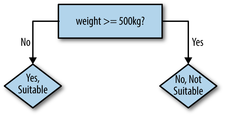
Figure 4-2. Robotâs first decision tree
The logic of the decision tree is easy to read and make some sense of: 500kg animals certainly sound unsuitable as pets. This rule predicts the correct value in five of nine cases. A quick glance suggests that we could improve the rule by lowering the weight threshold to 100kg. This gets six of nine examples correct. The heavy animals are now predicted correctly; the lighter animals are only partly correct.
So, a second decision can be constructed to further refine the
prediction for examples with weights less than 100kg. It would be good to pick a feature that changes some of the incorrect Yes predictions to No. For example, there is one small green animal, sounding suspiciously like a snake, that the robot could predict correctly by deciding on color, as shown in Figure 4-3.
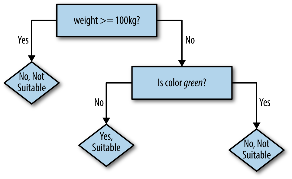
Figure 4-3. Robotâs next decision tree
Now, seven of nine examples are correct. Of course, decision rules could be added until all nine were correctly predicted. The logic embodied in the resulting decision tree would probably sound implausible when translated into common speech: âIf the animalâs weight is less than 100kg, and its color is brown instead of green, and it has fewer than 10 legs, then yes it is a suitable pet.â While perfectly fitting the given examples, a decision tree like this would fail to predict that a small, brown, four-legged wolverine is not a suitable pet. Some balance is needed to avoid this phenomenon, known as overfitting.
This is enough of an introduction to decision trees for us to begin using them with Spark. The remainder of the chapter will explore how to pick decision rules, how to know when to stop, and how to gain accuracy by creating a forest of trees.
Covtype Data Set
The data set used in this chapter is the well-known Covtype data set, available online as a compressed CSV-format data file, covtype.data.gz, and accompanying info file, covtype.info.
The data set records the types of forest-covering parcels of land in Colorado, USA. Itâs only a coincidence that the data set concerns real-world forests! Each example contains several features describing each parcel of landâlike its elevation, slope, distance to water, shade, and soil typeâalong with the known forest type covering the land. The forest cover type is to be predicted from the rest of the features, of which there are 54 in total.
This data set has been used in research and even a Kaggle competition. It is an interesting data set to explore in this chapter because it contains both categorical and numeric features. There are 581,012 examples in the data set, which does not exactly qualify as big data but is large enough to be manageable as an example and still highlight some issues of scale.
Preparing the Data
Thankfully, the data is already in a simple CSV format and does not require much cleansing or other preparation to be used with Spark MLlib. Later, it will be of interest to explore some transformations of the data, but it can be used as is to start.
The covtype.data file should be extracted and copied into HDFS. This chapter will assume that
the file is available at /user/ds/. Start spark-shell. You may again find it helpful to give
the shell a healthy amount of memory to work with, as building decision forests can be resource-intensive.
If you have the memory, specify --driver-memory 8g or similar.
CSV files contain fundamentally tabular data, organized into rows of columns. Sometimes these columns are given names in a header line, although thatâs not the case here. The column names are given in the companion file, covtype.info. Conceptually, each column of a CSV file has a type as wellâa number, a stringâbut a CSV file doesnât specify this.
Itâs natural to parse this data as a data frame because this is Sparkâs abstraction for tabular data, with a defined column schema, including column names and types. Spark has built-in support for reading CSV data, in fact:
valdataWithoutHeader=spark.read.option("inferSchema",true).option("header",false).csv("hdfs:///user/ds/covtype.data")...org.apache.spark.sql.DataFrame=[_c0:int,_c1:int...53morefields]
This code reads the input as CSV and does not attempt to parse the first line as a header of column names. It also requests that the type of each column be inferred by examining the data. It correctly infers that all of the columns are numbers, and more specifically, integers. Unfortunately it can only name the columns â_c0â and so on.
Looking at the column names, itâs clear that some features are indeed numeric. âElevationâ is an elevation in meters; âSlopeâ is measured in degrees. However, âWilderness_Areaâ is something different, because it is said to span four columns, each of which is a 0 or 1. In reality, âWilderness_Areaâ is a categorical value, not a numeric one.
These four columns are actually a
one-hot or 1-of-n encoding, in which one categorical feature
that takes on N distinct values becomes N numeric features, each taking on the value 0 or 1.
Exactly one of the N values has value 1, and the others are 0. For example, a categorical feature
for weather that can be cloudy, rainy, or clear would become three numeric features, where cloudy
is represented by 1,0,0; rainy by 0,1,0; and so on. These three numeric features might be thought
of as is_cloudy, is_rainy, and is_clear features.
Likewise, 40 of the columns are really one Soil_Type categorical feature.
This isnât the only possible way to encode a categorical feature as a number.
Another possible encoding simply assigns a distinct numeric value to each possible value of
the categorical feature. For example, cloudy may become 1.0, rainy 2.0, and so on.
The target itself, âCover_Typeâ, is a categorical value encoded as a value 1 to 7.
Be careful when encoding a categorical feature as a single numeric feature. The original categorical values have no ordering, but when encoded as a number, they appear to. Treating the encoded feature as numeric leads to meaningless results because the algorithm is effectively pretending that rainy is somehow greater than, and two times larger than, cloudy. Itâs OK as long as the encodingâs numeric value is not used as a number.
So we see both types of encodings of categorical features. It would have, perhaps, been simpler and more straightforward to not encode such features (and in two ways, no less), and instead simply include their values directly like âRawah Wilderness Area.â This may be an artifact of history; the data set was released in 1998. For performance reasons or to match the format expected by libraries of the day, which were built more for regression problems, data sets often contain data encoded in these ways.
In any event, before proceeding, it is useful to add column names to this DataFrame in order to make it easier to work with:
valcolNames=Seq("Elevation","Aspect","Slope","Horizontal_Distance_To_Hydrology","Vertical_Distance_To_Hydrology","Horizontal_Distance_To_Roadways","Hillshade_9am","Hillshade_Noon","Hillshade_3pm","Horizontal_Distance_To_Fire_Points")++((0until4).map(i=>s"Wilderness_Area_$i"))++((0until40).map(i=>s"Soil_Type_$i"))++Seq("Cover_Type")valdata=dataWithoutHeader.toDF(colNames:_*).withColumn("Cover_Type",$"Cover_Type".cast("double"))data.head...org.apache.spark.sql.Row=[2596,51,3,258,0,510,221,232,148,6279,1,0,0,0,...

++ concatenates collections
The wilderness- and soil-related columns are named âWilderness_Area_0â, âSoil_Type_0â, and a bit of Scala can generate these 44 names without having to type them all out. Finally, the target âCover_Typeâ column is cast to a double value upfront, because it will actually be necessary to consume it as a double rather than int in all Spark MLlib APIs. This will become apparent later.
You can call data.show() to see some rows of the data set, but the display is so wide that it will be difficult to read at all. data.head displays it as a raw Row object, which will be more readable in this case.
A First Decision Tree
In Chapter 3, we built a recommender model right away on all of the available data. This created a recommender that could be sense-checked by anyone with some knowledge of music: looking at a userâs listening habits and recommendations, we got some sense that it was producing good results. Here, that is not possible. We would have no idea how to make up a new 54-feature description of a new parcel of land in Colorado or what kind of forest cover to expect from such a parcel.
Instead, we must jump straight to holding out some data for purposes of evaluating the resulting model. Before, the AUC metric was used to assess the agreement between held-out listening data and predictions from recommendations. The principle is the same here, although the evaluation metric will be different: accuracy. The majorityâ90%âof the data will again be used for training, and later, weâll see that a subset of this training set will be held out for cross-validation (the CV set). The other 10% held out here is actually a third subset, a proper test set.
valArray(trainData,testData)=data.randomSplit(Array(0.9,0.1))trainData.cache()testData.cache()
The data needs a little more preparation to be used with a classifier in Spark MLlib. The input DataFrame contains many columns, each holding one feature that could be used to predict the target column. Spark MLlib requires all of the inputs to be collected into one column, whose value is a vector. This class is an abstraction for vectors in the linear algebra sense, and contains only numbers. For most intents and purposes, they work like a simple array of double values (floating-point numbers). Of course, some of the input features are conceptually categorical, even if theyâre all represented with numbers in the input. For now, weâll overlook this point and return to it later.
Fortunately, the VectorAssembler class can do this work:
importorg.apache.spark.ml.feature.VectorAssemblervalinputCols=trainData.columns.filter(_!="Cover_Type")valassembler=newVectorAssembler().setInputCols(inputCols).setOutputCol("featureVector")valassembledTrainData=assembler.transform(trainData)assembledTrainData.select("featureVector").show(truncate=false)...+-------------------------------------------------------------------...|featureVector...+-------------------------------------------------------------------...|(54,[0,1,2,3,4,5,6,7,8,9,13,15],[1863.0,37.0,17.0,120.0,18.0,90.0,2...|(54,[0,1,2,5,6,7,8,9,13,18],[1874.0,18.0,14.0,90.0,208.0,209.0,135....|(54,[0,1,2,3,4,5,6,7,8,9,13,18],[1879.0,28.0,19.0,30.0,12.0,95.0,20......
Its key parameters are the columns to combine into the feature vector, and the name of the new column containing the feature vector. Here, all columnsâexceptâthe target, of courseâare included as input features. The resulting DataFrame has a new âfeatureVectorâ column, as shown.
The output doesnât look exactly like a sequence of numbers,
but thatâs because this shows a raw representation of the vector, represented as a SparseVector
instance to save storage. Because most of the 54 values are 0, it only stores nonzero values and their indices.
This detail wonât matter in classification.
VectorAssembler is an example of Transformer within the current Spark MLlib âPipelinesâ API.
It transforms another DataFrame into a DataFrame, and is composable with other transformations into a pipeline. Later
in this chapter, these transformations will be connected into an actual Pipeline. Here, the transformation is just invoked directly, which is sufficient to build a first decision tree classifier model.
importorg.apache.spark.ml.classification.DecisionTreeClassifierimportscala.util.Randomvalclassifier=newDecisionTreeClassifier().setSeed(Random.nextLong()).setLabelCol("Cover_Type").setFeaturesCol("featureVector").setPredictionCol("prediction")valmodel=classifier.fit(assembledTrainData)println(model.toDebugString)...DecisionTreeClassificationModel(uid=dtc_29cfe1281b30)ofdepth5with63nodesIf(feature0<=3039.0)If(feature0<=2555.0)If(feature10<=0.0)If(feature0<=2453.0)If(feature3<=0.0)Predict:4.0Else(feature3>0.0)Predict:3.0...
Use random seed
Again, the essential configuration for the classifier consists of column names: the column containing the input feature vectors and the column containing the target value to predict. Because the model will later be used to predict new values of the target, it is given the name of a column to store predictions.
Printing a representation of the model shows some of its tree structure. It consists of a series of nested decisions about features, comparing feature values to thresholds. (Here, for historical reasons, the features are only referred to by number, not name, unfortunately.)
Decision trees are able to assess the importance of input features as part of their building process. That is, they can estimate how much each input feature contributes to making correct predictions. This information is simple to access from the model.
model.featureImportances.toArray.zip(inputCols).sorted.reverse.foreach(println)...(0.7931809106979147,Elevation)(0.050122380231328235,Horizontal_Distance_To_Hydrology)(0.030609364695664505,Wilderness_Area_0)(0.03052094489457567,Soil_Type_3)(0.026170212644908816,Hillshade_Noon)(0.024374024564392027,Soil_Type_1)(0.01670006142176787,Soil_Type_31)(0.012596990926899494,Horizontal_Distance_To_Roadways)(0.011205482194428473,Wilderness_Area_2)(0.0024194271152490235,Hillshade_3pm)(0.0018551637821715788,Horizontal_Distance_To_Fire_Points)(2.450368306995527E-4,Soil_Type_8)(0.0,Wilderness_Area_3)...
This pairs importance values (higher is better) with column names and prints them in order from most to least important. Elevation seems to dominate as the most important feature; most features are estimated to have virtually no importance when predicting the cover type!
The resulting DecisionTreeClassificationModel is itself a transformer because it can
transform a data frame containing feature vectors into a data frame also containing predictions.
For example, it might be interesting to see what the model predicts on the training data, and compare its prediction with the known correct cover type.
valpredictions=model.transform(assembledTrainData)predictions.select("Cover_Type","prediction","probability").show(truncate=false)...+----------+----------+------------------------------------------------...|Cover_Type|prediction|probability...+----------+----------+------------------------------------------------...|6.0|3.0|[0.0,0.0,0.03421818804589827,0.6318547696523378,...|6.0|4.0|[0.0,0.0,0.043440860215053764,0.283870967741935,...|6.0|3.0|[0.0,0.0,0.03421818804589827,0.6318547696523378,...|6.0|3.0|[0.0,0.0,0.03421818804589827,0.6318547696523378,......
Interestingly, the output also contains a âprobabilityâ column that gives the modelâs estimate of how likely it is that each possible outcome is correct. This shows that in these instances, itâs fairly sure the answer is 3 in several cases and quite sure the answer isnât 1.
Eagle-eyed readers might note that the probability vectors actually have eight values even though there are only seven possible outcomes. The vectorâs values at indices 1 to 7 do contain the probability of outcomes 1 to 7. However, there is also a value at index 0, which always shows as probability 0.0. This can be ignored, as 0 isnât even a valid outcome, as this says. Itâs a quirk of representing this information as a vector thatâs worth being aware of.
Based on this snippet, it looks like the model could use some work. Its predictions look like they are often wrong.
As with the ALS implementation, the DecisionTreeClassifier implementation has several hyperparameters
for which a value must be chosen, and theyâve all been left to defaults here.
Here, the test set can be used to produce an
unbiased evaluation of the expected accuracy of a model built with these default hyperparameters.
MulticlassClassificationEvaluator can compute
accuracy and other metrics that evaluate the quality of the modelâs predictions. Itâs an
example of an evaluator in Spark MLlib, which is responsible for assessing the quality
of an output DataFrame in some way.
importorg.apache.spark.ml.evaluation.MulticlassClassificationEvaluatorvalevaluator=newMulticlassClassificationEvaluator().setLabelCol("Cover_Type").setPredictionCol("prediction")evaluator.setMetricName("accuracy").evaluate(predictions)evaluator.setMetricName("f1").evaluate(predictions)...0.69763713855029890.6815943874214012
After being given the column containing the âlabelâ (target, or known correct output value) and the name of the column containing the prediction, it finds that the two match about 70% of the time. This is the accuracy of this classifier. It can compute other related measures, like the F1 score. For purposes here, accuracy will be used to evaluate classifiers.
This single number gives a good summary of the quality of the classifierâs output. Sometimes, however, it can be useful to look at the confusion matrix. This is a table with a row and a column for every possible value of the target. Because there are seven target category values, this is a 7Ã7 matrix, where each row corresponds to an actual correct value, and each column to a predicted value, in order. The entry at row i and column j counts the number of times an example with true category i was predicted as category j. So, the correct predictions are the counts along the diagonal and the predictions are everything else.
Fortunately, Spark provides support code to compute the confusion matrix. Unfortunately,
that implementation exists as part of the older MLlib APIs that operate on RDDs. However, thatâs
no big deal, because data frames and data sets can freely be turned into RDDs and used with
these older APIs. Here, MulticlassMetrics is appropriate for a data frame containing
predictions.
importorg.apache.spark.mllib.evaluation.MulticlassMetricsvalpredictionRDD=predictions.select("prediction","Cover_Type").as[(Double,Double)].rddvalmulticlassMetrics=newMulticlassMetrics(predictionRDD)multiclassMetrics.confusionMatrix...143125.041769.0164.00.00.00.05396.065865.0184360.03930.0102.039.00.0677.00.05680.025772.0674.00.00.00.00.021.01481.0973.00.00.00.087.07761.0648.00.069.00.00.00.06175.08902.0559.00.00.00.08058.024.050.00.00.00.010395.0
Convert to data set.

Convert to RDD.
Your values will be a little different. The process of building a decision tree includes some random choices that can lead to slightly different classifications.
Counts are high along the diagonal, which is good. However, there are certainly a number of misclassifications, and, for example, category 5 is never predicted at all.
Of course, itâs also possible to calculate something like a confusion matrix directly with the DataFrame API, using its more general operators. It is not necessary to rely on a specialized method anymore.
valconfusionMatrix=predictions.groupBy("Cover_Type").pivot("prediction",(1to7)).count().na.fill(0.0).orderBy("Cover_Type")confusionMatrix.show()...+----------+------+------+-----+---+---+---+-----+|Cover_Type|1|2|3|4|5|6|7|+----------+------+------+-----+---+---+---+-----+|1.0|143125|41769|164|0|0|0|5396||2.0|65865|184360|3930|102|39|0|677||3.0|0|5680|25772|674|0|0|0||4.0|0|21|1481|973|0|0|0||5.0|87|7761|648|0|69|0|0||6.0|0|6175|8902|559|0|0|0||7.0|8058|24|50|0|0|0|10395|+----------+------+------+-----+---+---+---+-----+
Replace null with 0
Microsoft Excel users may have recognized the problem as just like that of computing a pivot table. A pivot table groups values by two dimensions whose values become rows and columns of the output, and compute some aggregation within those groupings, like a count here. This is also available as a PIVOT function in several databases, and is supported by Spark SQL. Itâs arguably more elegant and powerful to compute it this way.
Although 70% accuracy sounds decent, itâs not immediately clear whether it is outstanding or poor. How well would a simplistic approach do to establish a baseline? Just as a broken clock is correct twice a day, randomly guessing a classification for each example would also occasionally produce the correct answer.
We could construct such a random âclassifierâ by picking a class at random in proportion to its prevalence in the training set. For example, if 30% of the training set were cover type 1, then the random classifier would guess â1â 33% of the time. Each classification would be correct in proportion to its prevalence in the test set. If 40% of the test set were cover type 1, then guessing â1â would be correct 40% of the time. Cover type 1 would then be guessed correctly 30% x 40% = 12% of the time and contribute 12% to overall accuracy. Therefore, we can evaluate the accuracy by summing these products of probabilities:
importorg.apache.spark.sql.DataFramedefclassProbabilities(data:DataFrame):Array[Double]={valtotal=data.count()data.groupBy("Cover_Type").count().orderBy("Cover_Type").select("count").as[Double].map(_/total).collect()}valtrainPriorProbabilities=classProbabilities(trainData)valtestPriorProbabilities=classProbabilities(testData)trainPriorProbabilities.zip(testPriorProbabilities).map{case(trainProb,cvProb)=>trainProb*cvProb}.sum...0.3771270477245849
Count by category
Order counts by category

To data set

Sum products of pairs in training, test sets
Random guessing achieves 37% accuracy then, which makes 70% seem like a good result after all. But this result was achieved with default hyperparameters. We can do even better by exploring what these actually mean for the tree-building process.
Decision Tree Hyperparameters
In Chapter 3, the ALS algorithm exposed several hyperparameters whose values we had to choose by building models with various combinations of values and then assessing the quality of each result using some metric. The process is the same here, although the metric is now multiclass accuracy instead of AUC. The hyperparameters controlling how the treeâs decisions are chosen will be quite different as well: maximum depth, maximum bins, impurity measure, and minimum information gain.
Maximum depth simply limits the number of levels in the decision tree. It is the maximum number of chained decisions that the classifier will make to classify an example. It is useful to limit this to avoid overfitting the training data, as illustrated previously in the pet store example.
The decision tree algorithm is responsible for coming up with potential decision rules to try
at each level, like the weight >= 100 or weight >= 500 decisions in the pet store example.
Decisions are always of the same form: for numeric features, decisions are of the form feature >= value; and for categorical features, they are of the form feature in (value1, value2, â¦). So, the set of decision rules
to try is really a set of values to plug in to the decision rule. These are referred to as
âbinsâ in the Spark MLlib implementation. A larger number of bins requires more processing
time but might lead to finding a more optimal decision rule.
What makes a decision rule good? Intuitively, a good rule would meaningfully distinguish examples by target category value. For example, a rule that divides the Covtype data set into examples with only categories 1â3 on the one hand and 4â7 on the other would be excellent because it clearly separates some categories from others. A rule that resulted in about the same mix of all categories as are found in the whole data set doesnât seem helpful. Following either branch of such a decision leads to about the same distribution of possible target values, and so doesnât really make progress toward a confident classification.
Put another way, good rules divide the training dataâs target values into relatively homogeneous, or âpure,â subsets. Picking a best rule means minimizing the impurity of the two subsets it induces. There are two commonly used measures of impurity: Gini impurity and entropy.
Gini impurity is directly related to the accuracy of the random-guess classifier. Within a subset, it is the probability that a randomly chosen classification of a randomly chosen example (both according to the distribution of classes in the subset) is incorrect. This is the sum of products of proportions of classes, but with themselves and subtracted from 1. If a subset has N classes and pi is the proportion of examples of class i, then its Gini impurity is given in the Gini impurity equation:
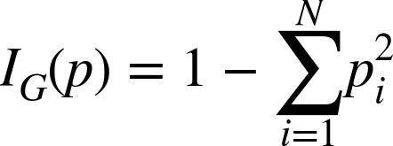
If the subset contains only one class, this value is 0 because it is completely âpure.â When there are N classes in the subset, this value is larger than 0 and is largest when the classes occur the same number of timesâmaximally impure.
Entropy is another measure of impurity, borrowed from information theory. Its nature is more difficult to explain, but it captures how much uncertainty the collection of target values in the subset implies about predictions for data that falls in that subset. A subset containing one class suggests that the outcome for the subset is completely certain and has 0 entropyâno uncertainty. A subset containing one of each possible class, on the other hand, suggests a lot of uncertainty about predictions for that subset because data have been observed with all kinds of target values. This has high entropy. Hence, low entropy, like low Gini impurity, is a good thing. Entropy is defined by the entropy equation:
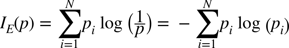
Interestingly, uncertainty has units. Because the logarithm is the natural log (base e), the units are nats, the base-e counterpart to more familiar bits (which we can obtain by using log base 2 instead). It really is measuring information, so itâs also common to talk about the information gain of a decision rule when using entropy with decision trees.
One or the other measure may be a better metric for picking decision rules in a given data set. They are, in a way, similar. Both involve a weighted average: a sum over values weighted by pi. The default in Sparkâs implementation is Gini impurity.
Finally, minimum information gain is a hyperparameter that imposes a minimum information gain, or decrease in impurity, for candidate decision rules. Rules that do not improve the subsets impurity enough are rejected. Like a lower maximum depth, this can help the model resist overfitting because decisions that barely help divide the training input may in fact not helpfully divide future data at all.
Tuning Decision Trees
Itâs not obvious from looking at the data which impurity measure leads to better accuracy, or what maximum depth or number of bins is enough without being excessive. Fortunately, as in Chapter 3, itâs simple to let Spark try a number of combinations of these values and report the results.
First, itâs necessary to set up a pipeline encapsulating the same
two steps above. Creating the VectorAssembler and DecisionTreeClassifier and chaining
these two Transformers together results in a single Pipeline object that represents
these two operations together as one operation:
importorg.apache.spark.ml.PipelinevalinputCols=trainData.columns.filter(_!="Cover_Type")valassembler=newVectorAssembler().setInputCols(inputCols).setOutputCol("featureVector")valclassifier=newDecisionTreeClassifier().setSeed(Random.nextLong()).setLabelCol("Cover_Type").setFeaturesCol("featureVector").setPredictionCol("prediction")valpipeline=newPipeline().setStages(Array(assembler,classifier))
Naturally, pipelines can be much longer and more complex. This is about as simple as it gets.
Now we can also define the combinations of hyperparameters that should be tested using the
Spark ML APIâs built-in support, ParamGridBuilder. Itâs also time to define the evaluation
metric that will be used to pick the âbestâ hyperparameters, and that is again
MulticlassClassificationEvaluator here.
importorg.apache.spark.ml.tuning.ParamGridBuildervalparamGrid=newParamGridBuilder().addGrid(classifier.impurity,Seq("gini","entropy")).addGrid(classifier.maxDepth,Seq(1,20)).addGrid(classifier.maxBins,Seq(40,300)).addGrid(classifier.minInfoGain,Seq(0.0,0.05)).build()valmulticlassEval=newMulticlassClassificationEvaluator().setLabelCol("Cover_Type").setPredictionCol("prediction").setMetricName("accuracy")
This means that a model will be built and evaluated for two values of four hyperparameters. Thatâs 16 models. Theyâll be evaluated by multiclass accuracy. Finally, TrainValidationSplit brings these components togetherâthe pipeline that makes models, model evaluation metrics, and hyperparameters to tryâand can run the evaluation on the training data. Itâs worth noting that CrossValidator could be
used here as well to perform full k-fold cross-validation, but it is k times more expensive and doesnât add as much value in the presence of big data. So, TrainValidationSplit is used here.
importorg.apache.spark.ml.tuning.TrainValidationSplitvalvalidator=newTrainValidationSplit().setSeed(Random.nextLong()).setEstimator(pipeline).setEvaluator(multiclassEval).setEstimatorParamMaps(paramGrid).setTrainRatio(0.9)valvalidatorModel=validator.fit(trainData)
This will take minutes or more, depending on your hardware, because itâs building and evaluating many models.
Note the train ratio parameter is set to 0.9. This means that the training data is actually
further subdivided by TrainValidationSplit into 90%/10% subsets. The former is used
for training each model. The remaining 10% of the input is held out as a cross-validation
set to evaluate the model. If itâs already holding out some data for evaluation, then why did we hold out 10% of the
original data as a test set?
If the purpose of the CV set was to evaluate parameters that fit to the training set, then the purpose of the test set is to evaluate hyperparameters that were âfitâ to the CV set. That is, the test set ensures an unbiased estimate of the accuracy of the final, chosen model and its hyperparameters.
Say that the best model chosen by this process exhibits 90% accuracy on the CV set. It seems reasonable to expect it will exhibit 90% accuracy on future data. However, thereâs an element of randomness in how these models are built. By chance, this model and evaluation could have turned out unusually well. The top model and evaluation result could have benefited from a bit of luck, so its accuracy estimate is likely to be slightly optimistic. Put another way, hyperparameters can overfit too.
To really assess how well this best model is likely to perform on future examples, we need to evaluate it on examples that were not used to train it. But we also need to avoid examples in the CV set that were used to evaluate it. That is why a third subset, the test set, was held out.
The result of the validator contains the best model it found. This itself is a representation of the best overall pipeline it found, because we provided an instance of a pipeline to run. In order to query the parameters chosen by DecisionTreeClassifier, itâs necessary to
manually extract DecisionTreeClassificationModel from the resulting PipelineModel, which is the final stage in the pipeline.
importorg.apache.spark.ml.PipelineModelvalbestModel=validatorModel.bestModelbestModel.asInstanceOf[PipelineModel].stages.last.extractParamMap...{dtc_9136220619b4-cacheNodeIds:false,dtc_9136220619b4-checkpointInterval:10,dtc_9136220619b4-featuresCol:featureVector,dtc_9136220619b4-impurity:entropy,dtc_9136220619b4-labelCol:Cover_Type,dtc_9136220619b4-maxBins:40,dtc_9136220619b4-maxDepth:20,dtc_9136220619b4-maxMemoryInMB:256,dtc_9136220619b4-minInfoGain:0.0,dtc_9136220619b4-minInstancesPerNode:1,dtc_9136220619b4-predictionCol:prediction,dtc_9136220619b4-probabilityCol:probability,dtc_9136220619b4-rawPredictionCol:rawPrediction,dtc_9136220619b4-seed:159147643}
This contains a lot of information about the fitted model, but it also tells us that âentropyâ apparently worked best as the impurity measure and that a max depth of 20 was not surprisingly better than 1. It might be surprising that the best model was fit with just 40 bins, but this is probably a sign that 40 was âplentyâ rather than âbetterâ than 300. Lastly, no minimum information gain was better than a small minimum, which could imply that the model is more prone to underfit than overfit.
You may wonder if it is possible to see the accuracy that each of the models achieved for each combination of hyperparameters. The hyperparameters as well as the evaluations are exposed by getEstimatorParamMaps and validationMetrics, respectively. They can be combined to display all of the parameter combinations sorted by metric value:
valvalidatorModel=validator.fit(trainData)valparamsAndMetrics=validatorModel.validationMetrics.zip(validatorModel.getEstimatorParamMaps).sortBy(-_._1)paramsAndMetrics.foreach{case(metric,params)=>println(metric)println(params)println()}...0.9138483377774368{dtc_3e3b8bb692d1-impurity:entropy,dtc_3e3b8bb692d1-maxBins:40,dtc_3e3b8bb692d1-maxDepth:20,dtc_3e3b8bb692d1-minInfoGain:0.0}0.9122369506416774{dtc_3e3b8bb692d1-impurity:entropy,dtc_3e3b8bb692d1-maxBins:300,dtc_3e3b8bb692d1-maxDepth:20,dtc_3e3b8bb692d1-minInfoGain:0.0}...
What was the accuracy that this model achieved on the CV set? And finally, what accuracy does the model achieve on the test set?
validatorModel.validationMetrics.maxmulticlassEval.evaluate(bestModel.transform(testData))...0.91384833777743680.9139978718291971
bestModel is a complete pipeline.
The results are both about 91%. It happens that the estimate from the CV set was pretty fine to begin with. In fact, it is not usual for the test set to show a very different result.
This is an interesting point at which to revisit the issue of overfitting. As discussed previously, itâs possible to build a decision tree so deep and elaborate that it fits the given training examples very well or perfectly but fails to generalize to other examples because it has fit the idiosyncrasies and noise of the training data too closely. This is a problem common to most machine learning algorithms, not just decision trees.
When a decision tree has overfit, it will exhibit high accuracy when run
on the same training data that it fit the model to, but low accuracy on other examples.
Here, the final modelâs accuracy was about 91% on other, new
examples. Accuracy can just as easily be evaluated over the same data that the model was trained on,
trainData. This gives an accuracy of about 95%.
The difference is not large but suggests that the decision tree has overfit the training data to some extent. A lower maximum depth might be a better choice.
Categorical Features Revisited
So far, the code examples have implicitly treated all input features as if theyâre numeric (though âCover_Typeâ, despite being encoded as numeric, has actually been correctly treated as a categorical value.) This isnât exactly wrong, because the categorical features here are one-hot encoded as several binary 0/1 values. Treating these individual features as numeric turns out to be fine, because any decision rule on the ânumericâ features will choose thresholds between 0 and 1, and all are equivalent since all values are 0 or 1.
Of course, this encoding forces the decision tree algorithm to consider the values of the underlying categorical features individually. Because features like soil type are broken down into many features, and because decision trees treat features individually, it is harder to relate information about related soil types.
For example, nine different soil types are actually part of the Leighcan family, and they may be related in ways that the decision tree can exploit. If soil type were encoded as a single categorical feature with 40 soil values, then the tree could express rules like âif the soil type is one of the nine Leighton family typesâ directly. However, when encoded as 40 features, the tree would have to learn a sequence of nine decisions on soil type to do the same, this expressiveness may lead to better decisions and more efficient trees.
However, having 40 numeric features represent one 40-valued categorical feature increases memory usage and slows things down.
What about undoing the one-hot encoding? This would replace, for example, the four columns encoding wilderness type with one column that encodes the wilderness type as a number between 0 and 3, like âCover_Typeâ.
importorg.apache.spark.sql.functions._defunencodeOneHot(data:DataFrame):DataFrame={valwildernessCols=(0until4).map(i=>s"Wilderness_Area_$i").toArrayvalwildernessAssembler=newVectorAssembler().setInputCols(wildernessCols).setOutputCol("wilderness")valunhotUDF=udf((vec:Vector)=>vec.toArray.indexOf(1.0).toDouble)valwithWilderness=wildernessAssembler.transform(data).drop(wildernessCols:_*).withColumn("wilderness",unhotUDF($"wilderness"))valsoilCols=(0until40).map(i=>s"Soil_Type_$i").toArrayvalsoilAssembler=newVectorAssembler().setInputCols(soilCols).setOutputCol("soil")soilAssembler.transform(withWilderness).drop(soilCols:_*).withColumn("soil",unhotUDF($"soil"))}
Note UDF definition
Drop one-hot columns; no longer needed
Overwrite column with numeric one of same name
Here VectorAssembler is deployed to combine the 4 and 40 wilderness and soil type columns into
two Vector columns. The values in these Vectors are all 0, except for one location
that has a 1. Thereâs no simple DataFrame function for this, so we have to define our own UDF that can be used to operate on columns. This turns these two new columns into numbers of just the type we need.
From here, nearly the same process as above can be used to tune the hyperparameters of a decision tree model built on this data and to choose and evaluate a best model. Thereâs one important difference, however. The two new numeric columns have nothing about them that indicates theyâre actually an encoding of categorical values. To treat them as numbers would be wrong, as their ordering is meaningless. However, it would silently succeed; the information in these features would be all but lost though.
Internally Spark MLlib can store additional metadata about each column. The details of this
data are generally hidden from the caller, but includes information such as whether the
column encodes a categorical value and how many distinct values it takes on. In order to
add this metadata, itâs necessary to put the data through VectorIndexer. Its job is to turn
input into properly labeled categorical feature columns. Although we did much of the work already
to turn the categorical features into 0-indexed values, VectorIndexer will take care of the
metadata.
We need to add this stage to the Pipeline:
importorg.apache.spark.ml.feature.VectorIndexervalinputCols=unencTrainData.columns.filter(_!="Cover_Type")valassembler=newVectorAssembler().setInputCols(inputCols).setOutputCol("featureVector")valindexer=newVectorIndexer().setMaxCategories(40).setInputCol("featureVector").setOutputCol("indexedVector")valclassifier=newDecisionTreeClassifier().setSeed(Random.nextLong()).setLabelCol("Cover_Type").setFeaturesCol("indexedVector").setPredictionCol("prediction")valpipeline=newPipeline().setStages(Array(assembler,indexer,classifier))
>= 40 because soil has 40 values
The approach assumes that the training set contains all possible values of each of the
categorical features at least once. That is, it works correctly only if all 4 soil values
and all 40 wilderness values appear in the training set so that all possible values get a
mapping. Here, that happens to be true, but may not be for small training sets of data in which
some labels appear very infrequently. In those cases, it could be necessary to manually create and add
a VectorIndexerModel with the complete value mapping supplied manually.
Aside from that, the process is the same as before. You should find that it chose a similar best model but that accuracy on the test set is about 93%. By treating categorical features as actual categorical features, the classifier improved its accuracy by almost 2%.
Random Decision Forests
If you have been following along with the code examples, you may have noticed that your results differ slightly from those presented in the code listings in the book. That is because there is an element of randomness in building decision trees, and the randomness comes into play when youâre deciding what data to use and what decision rules to explore.
The algorithm does not consider every possible decision rule at every level. To do so would take an incredible amount of time. For a categorical feature over N values, there are 2Nâ2 possible decision rules (every subset except the empty set and entire set). For even moderately large N, this would create billions of candidate decision rules.
Instead, decision trees use several heuristics to determine which few rules to actually consider. The process of picking rules also involves some randomness; only a few features picked at random are looked at each time, and only values from a random subset of the training data. This trades a bit of accuracy for a lot of speed, but it also means that the decision tree algorithm wonât build the same tree every time. This is a good thing.
Itâs good for the same reason that the âwisdom of the crowdsâ usually beats individual predictions. To illustrate, take this quick quiz: How many black taxis operate in London?
Donât peek at the answer; guess first.
I guessed 10,000, which is well off the correct answer of about 19,000. Because I guessed low, youâre a bit more likely to have guessed higher than I did, and so the average of our answers will tend to be more accurate. Thereâs that regression to the mean again. The average guess from an informal poll of 13 people in the office was indeed closer: 11,170.
A key to this effect is that the guesses were independent and didnât influence one another. (You didnât peek, did you?) The exercise would be useless if we had all agreed on and used the same methodology to make a guess, because the guesses would have been the same answerâthe same potentially quite wrong answer. It would even have been different and worse if Iâd merely influenced you by stating my guess upfront.
It would be great to have not one tree, but many trees, each producing reasonable but different and independent estimations of the right target value. Their collective average prediction should fall close to the true answer, more than any individual treeâs does. Itâs the randomness in the process of building that helps create this independence. This is the key to random decision forests.
Randomness is injected by building many trees, each of which sees a different random subset of dataâand even of features. This makes the forest as a whole less prone to overfitting. If a particular feature contains noisy data or is deceptively predictive only in the training set, then most trees will not consider this problem feature most of the time. Most trees will not fit the noise and will tend to âoutvoteâ the trees that have fit the noise in the forest.
The prediction of a random decision forest is simply a weighted average of the treesâ predictions. For a categorical target, this can be a majority vote or the most probable value based on the average of probabilities produced by the trees. Random decision forests, like decision trees, also support regression, and the forestâs prediction in this case is the average of the number predicted by each tree.
While random decision forests are a more powerful and complex classification technique, the
good news is that itâs virtually no different to use it in the pipeline that has been
developed in this chapter. Simply drop in a RandomForestClassifier in place of DecisionTreeClassifier and proceed
as before. Thereâs really no more code or API to understand in order to use it.
importorg.apache.spark.ml.classification.RandomForestClassifiervalclassifier=newRandomForestClassifier().setSeed(Random.nextLong()).setLabelCol("Cover_Type").setFeaturesCol("indexedVector").setPredictionCol("prediction")
Note that this classifier has another hyperparameter: the number of trees to build. Like the max bins hyperparameter, higher values should give better results up to a point. The cost, however, is that building many trees of course takes many times longer than building one.
The accuracy of the best random decision forest model produced from a similar tuning process is 95% off the batâabout 2% better already, although viewed another way, thatâs a 28% reduction in the error rate over the best decision tree built previously, from 7% down to 5%. You may do better with further tuning.
Incidentally, at this point we have a more reliable picture of feature importance:
importorg.apache.spark.ml.classification.RandomForestClassificationModelvalforestModel=bestModel.asInstanceOf[PipelineModel].stages.last.asInstanceOf[RandomForestClassificationModel]forestModel.featureImportances.toArray.zip(inputCols).sorted.reverse.foreach(println)...(0.28877055118903183,Elevation)(0.17288279582959612,soil)(0.12105056811661499,Horizontal_Distance_To_Roadways)(0.1121550648692802,Horizontal_Distance_To_Fire_Points)(0.08805270405239551,wilderness)(0.04467393191338021,Vertical_Distance_To_Hydrology)(0.04293099150373547,Horizontal_Distance_To_Hydrology)(0.03149644050848614,Hillshade_Noon)(0.028408483578137605,Hillshade_9am)(0.027185325937200706,Aspect)(0.027075578474331806,Hillshade_3pm)(0.015317564027809389,Slope)
Random decision forests are appealing in the context of big data because trees are supposed to be built independently, and big data technologies like Spark and MapReduce inherently need data-parallel problems, where parts of the overall solution can be computed independently on parts of the data. The fact that trees can, and should, train on only a subset of features or input data makes it trivial to parallelize building the trees.
Making Predictions
Building a classifier, while an interesting and nuanced process, is not the end goal. The goal is to make predictions. This is the payoff, and it is comparatively quite easy.
The resulting âbest modelâ is actually a whole pipeline of operations,
which encapsulate how input is transformed for use with the model and includes the model itself, which can make predictions. It can operate on a data frame of new input. The only difference from the data DataFrame we started with is that it lacks the âCover_Typeâ column. When weâre making predictionsâespecially about the future, says Mr. Bohrâthe output is of course not known.
To prove it, try dropping the âCover_Typeâ from the test data input and obtaining a prediction:
bestModel.transform(unencTestData.drop("Cover_Type")).select("prediction").show()...+----------+|prediction|+----------+|6.0|+----------+
The result should be 6.0, which corresponds to class 7 (the original feature was 1-indexed) in the original Covtype data set. The predicted cover type for the land described in this example is Krummholz. Obviously.
Where to Go from Here
This chapter introduced two related and important types of machine learning, classification and regression, along with some foundational concepts in building and tuning models: features, vectors, training, and cross-validation. It demonstrated how to predict a type of forest cover from things like location and soil type using the Covtype data set, with decision trees and forests implemented in Spark MLlib.
As with recommenders in Chapter 3, it could be useful to continue exploring the effect of hyperparameters on accuracy. Most decision tree hyperparameters trade time for accuracy: more bins and trees generally produce better accuracy but hit a point of diminishing returns.
The classifier here turned out to be very accurate. Itâs unusual to achieve more than 95% accuracy. In general, you will achieve further improvements in accuracy by including more features or transforming existing features into a more predictive form. This is a common, repeated step in iteratively improving a classifier model. For example, for this data set, the two features encoding horizontal and vertical distance-to-surface-water features could produce a third feature: straight-line distance-to-surface-water features. This might turn out to be more useful than either original feature. Or, if it were possible to collect more data, we might try adding new information like soil moisture in order to improve classification.
Of course, not all prediction problems in the real world are exactly like
the Covtype data set. For example, some problems require predicting a continuous numeric value,
not a categorical value. Much of the same analysis and code applies to this type of
regression problem; the RandomForestRegressor class will be of use in this case.
Furthermore, decision trees and forests are not the only classification or regression algorithms, and not the only ones implemented in Spark MLlib. For classification, it includes implementations of:
Yes, logistic regression is a classification technique. Underneath the hood, it classifies by predicting a continuous function of a class probability. This detail is not necessary to understand.
Each of these algorithms operates quite differently from decision trees and forests. However, many elements are the same: they plug into a Pipeline and operate on columns in a data frame, and have hyperparameters that you must select using training, cross-validation, and test subsets of the input data. The same general principles, with these other algorithms, can also be deployed to model classification and regression problems.
These have been examples of supervised learning. What happens when some, or all, of the target values are unknown? The following chapter will explore what can be done in this situation.
Get Advanced Analytics with Spark, 2nd Edition now with the O’Reilly learning platform.
O’Reilly members experience books, live events, courses curated by job role, and more from O’Reilly and nearly 200 top publishers.

