42 Applied calculus of variations for engineers
-3
-2
-1
0
1
2
3
-3
-2
-1
0
1
2
3
-30
-20
-10
0
10
20
30
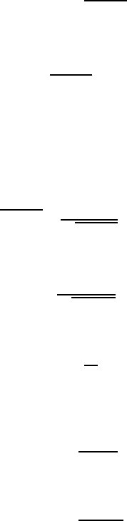
FIGURE 3.1 Saddle surface
the equation.
When a minimal surface is sought in a parametric form
r
= x(u, v)i + y(u, v)j + z(u, v)k.
the variational problem becomes
I(r
)=
D
EF −G
2
dA,
where the so-called first fundamental quantities are defined as
E(u, v)=(r
u
)
2
,
F (u, v)=r
u
r
v
,
and
G(u, v)=(r
v
)
2
.
The solution may be obtained from the differential equation
∂
∂u
Fr
u
− Gr
v
√
EF − G
2
+
∂
∂v
Er
v
− Gr
u
√
EF −G
2
=0.