Digital Communications

Appendix B: Gaussian Q Function

B.1 Gaussian Q‐Function

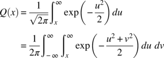
The Gaussian Q‐function, which is defined by

(B.1)

represents the area under the tail (between x and ∞) of a zero‐mean and unit variance Gaussian pdf f_Z(z) (see Figure B.1). Since the area under a pdf is equal to unity, Q(−∞) = 1 and Q(∞) = 0. Owing to the symmetry of the Gaussian pdf with respect to the origin, Q(0) = 1/2 and

(B.2)

Figure B.1 Gaussian Q‐Function and the Gaussian (Normal) Pdf with Zero‐Mean and Unity Variance.

The Craig’s definition of the Q‐function [1] can easily be derived from (B.1) as follows:

(B.3)

If we make a transformation of Cartesian coordinates to polar coordinates as and inserting into (B.3) (see Figure B.2), one gets

(B.4)

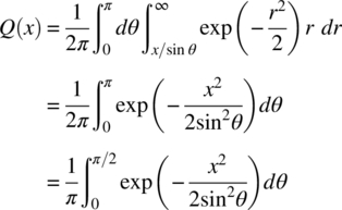
Figure B.2 Coordinate Transformation For Deriving the Craig’s Formula For ...