Digital Signal Processing Using Matlab

2.2. Solved exercises

EXERCISE 2.1.

The MATLAB code below generates and plots some basic discrete-time signals.

subplot (3,3,1);
stem([1;zeros (49,1)]);
title('Dirac pulse')
subplot(3,3,2); stem(ones(50,1));
title(' Step function')
subplot (3,3,3);
stem ([ones (1,5),zeros(1,3)])
title(' Rectangular pulse')
subplot (3,3,4);
stem(sin(2*pi/8*(0:15)) )
title('Sinusoidal signal')
subplot (3,3,5); stem(sinc(0:0.25:8)) ;
title('“Sinc” signal')
subplot (3,3,6); stem(exp(- (0:15)));
title('e^-^n signal')
subplot (3,3,7);
stem(pow2(-0.5*(0:15)))
title('2^-^0^.^5^n signal')
subplot(3,3,8); stem(3.^(0:15));
title('3^n signal')
subplot(3,3,9); stem (randn(1,16));
title('Gaussian random signal')

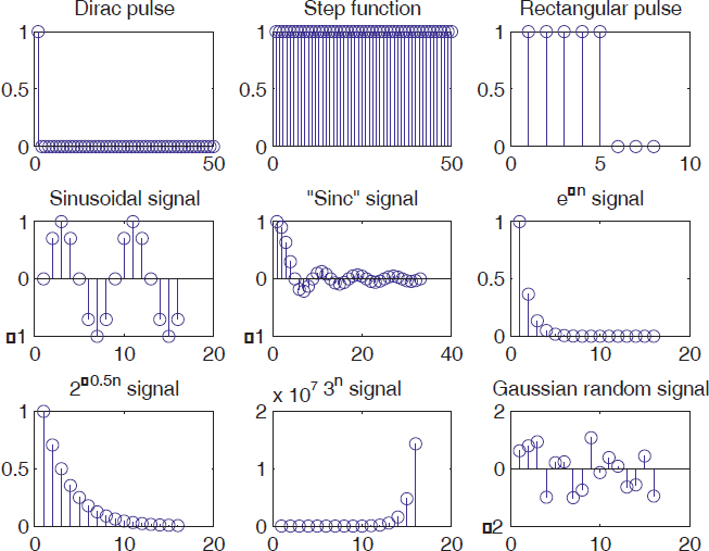
Figure 2.1. Examples of discrete-time signals

EXERCISE 2.2.

Generate the following signal:

x(n) = K · exp[c · n],

where: K = 2, c = −1/12 + jπ/6, n N and n = 0..40 .

c = -(1/12) + (pi/6)*i;
K = 2; n = 0:40;
x = K*exp(c*n);
subplot (2,1,1); stem(n, real(x));
xlabel('Iime index n');
ylabel('Amplitude');
title('Real part');
subplot (2,1,2); stem, (n, imag(x));
xlabel('Time index n');
ylabel('Amplitude');
title('Imaginary part');

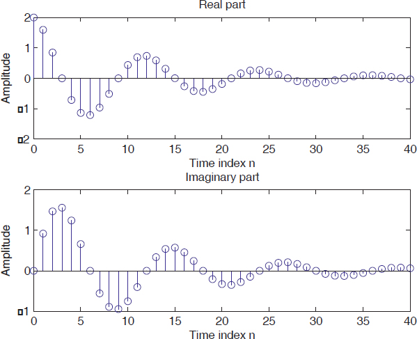
Figure 2.2. Real and imaginary parts of a complex discrete-time signal

K