Digital Signal Processing Using Matlab

3.3. Exercises

EXERCISE 3.8.

Consider a zero-mean random Gaussian signal with the variance 3 at the input of the following systems:

• – thresholder;
• – rectifier;
• – quadratic filter.

Determine the pdf of the output signals and estimate their 1^st and 2^nd order moments.

EXERCISE 3.9.

Go back to exercise 3.4 and consider a constant initial phase, but a uniformly distributed random amplitude, with the mean value 3 and standard deviation 0.5. Comment on the 2^nd order stationarity of the new random process? Does the ergodicity have any sense in this case?

EXERCISE 3.10.

Write a MATLAB code for generating N samples of a random variable X having the following pdf:

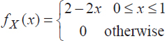
Find out the mean value and the variance of this random variable.

EXERCISE 3.11.

A linear system such as the one used in exercise 3.5 is driven by a zero-mean white uniform noise having a standard deviation of 5. Calculate and comment on the output signal pdf for ρ values between 0 and 0.999, such as ρ = 0.001, ρ = 0.01, ρ = 0.1, ρ = 0.5 and ρ = 0.95.

Can you explain the different obtained pdfs? Calculate the mean values and the variances of all variables. Let ρ = -0.7 and comment on the mean value and the variance.

EXERCISE 3.12.

Simulate the effect of decreasing the number of quantification bits for a 32 bit coded signal. Plot the quantification error and its pdf.

Calculate the SNR and demonstrate that it increases with 6 dB ...