Digital Signal Processing Using Matlab

6.2. Solved exercises

EXERCISE 6.1.

1. Write a MATLAB code to verify the linearity of system , represented by the transfer function:

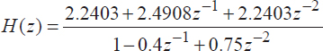
Consider for this two different signals x and y and demonstrate the following relationship: .

clf; n = 0:40; a = 2;b = -3;
x1 = cos(2*pi*0.1*n); x2 = cos(2*pi*0.4*n); x = a*x1 + b*x2;
num = [2.2403 2.4908 2.2403]; den = [1 -0.4 0.75];
ic = [0 0]; % set the initial conditions to zero
y1 = filter(num,den,x1,ic); %Calculation of the output signal y1[n]
y2 = filter(num,den,x2, ic); %Calculation of the output signal y2[n]
y = filter(num,den,x,ic); %Calculation of the output signal y[n]
yt = a*y1 + b*y2; d = y - yt; %Calculation of the error signal d[n]
% Plotting the error and the output signals
subplot(3,1,1); stem(n,y); ylabel('Amplitude');
title('Output corresponding to: a\cdot x_{1}[n] + b\cdot x_{2} [n]');
subplot (3,1,2); stem(n,yt) ; ylabel('Amplitude');
title('Output calculated as: a\cdot y_{1}[n] + b\cdot y_{2} [n]');
subplot(3,1,3); stem(n,d); xlabel('Time index n');
ylabel('Amplitude'); title('Error signal');

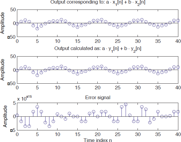
Figure 6.1. Linearity of the convolution ...