CHAPTER 5
WINDOWING AND LOCALIZATION
5.1 OVERVIEW: NONLOCALITY OF THE DFT
Let’s begin with an example.
![]() EXAMPLE 5.1
EXAMPLE 5.1
Consider two different audio signals f(t) and g(t) defined on 0 ≤ t ≤ 1, given by
![]()
and

Both are composed of the same two basic waveforms, sin(2π(96)t) and sin(2π(235)t). In f the waveforms are present throughout, while in g each waveform is present for exactly half of the time interval [0, 1],
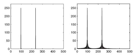
Let us sample each at 1000 Hertz to produce sample vectors f and g, and then compute the DFT of each sampled signal. The magnitude of each is plotted in Figure 5.1, DFT(f) on the left and DFT(g) on the right, where in each graph the horizontal index k corresponds to k Hertz. It’s obvious from the plots that each signal contains dominant frequencies near 96 and 235 Hertz, and the magnitude of the DFT’s are otherwise fairly similar. But the signals f(t) and g(t) are quite different in the time domain, a fact that is difficult to glean from the DFT graphs.
FIGURE 5.1 Magnitude of DFT for f (left) and g (right).

This example illustrates one of the shortcomings of traditional Fourier ...

