Discrete Stochastic Processes and Optimal Filtering

Examples treated using Matlab software

First example of Kalman filtering

The objective is to estimate an unknown constant drowned in noise.

This constant is measured using a noise sensor.

The noise is centered, Gaussian and of variance equal to 1.

The initial conditions are equal to 0 for the estimate and equal to 1 for the variance of the estimation error.

clear
t=0:500;
R0=1;
constant=rand(1);
n1=randn(size(t));
y=constant+n1;

subplot(2,2,1)
%plot(t,y(1,:));
plot(t,y,’k’);% in B&W

grid
title(‘sensor’)
xlabel(‘time’)
axis([0 500 -max(y(1,:)) max(y(1,:))])

R=R0*std(n1)^2;% variance of noise measurement

P(1)=1;%initial conditions on variance of error estimation
x(1)=0;

for i=2:length(t)
 K=P(i-1)*inv(P(i-1)+R);
 x(i)=x(i-1)+K*(y(:,i)-x(i-1));
 P(i)=P(i-1)-K*P(i-1);
end
err=constant-x;
subplot(2,2,2)
plot(t,err,’k’);
grid
title(‘error’);
xlabel(‘time’)
axis([0 500 -max(err) max(err)])

subplot(2,2,3)
plot(t,x,’k’,t,constant,’k’);% in W&B
title(‘x estimated’)
xlabel(‘time’)
axis([0 500 0 max(x)])
grid

subplot(2,2,4)
plot(t,P,’k’);% in W&B
grid,axis([0 100 0 max(P)])
title(‘variance error estimation’)
xlabel(‘time’)

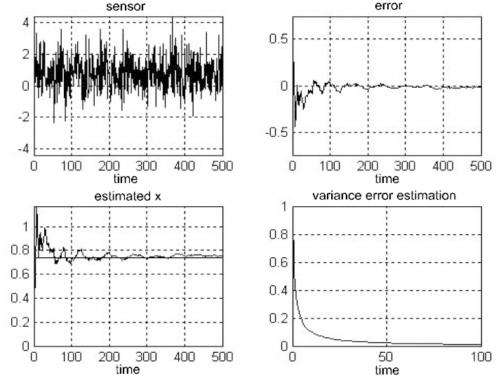
Figure 7.3. Line graph of measurement, error, best filtration and variance of error

Second example of Kalman filtering

The objective of this example is to extract a dampened sine curve of the noise.

The state vector is a two component column vector:

The system noise is centered, ...