Chapter 4. Explainability for Image Data
Introduced in the 1980s, convolutional neural networks (CNNs), like DNNs, remained unused until the advent of modern ML, at which point they quickly became the backbone of contemporary solutions for computer vision problems. Since then, deep learning models based on CNNs have enabled unprecedented breakthroughs in many computer vision tasks ranging from image classification and semantic segmentation to image captioning and visual question answering, at times achieving near human-level performance. Nowadays, you can find sophisticated computer vision models being used to design smart cities, monitor livestock or crop development, build self-driving cars, or identify eye disease or lung cancer.
As the number of these intelligent systems relying on image models continues to grow, the role of explainability in analyzing and understanding these systems has become more important than ever. Unfortunately, when these highly complex systems fail, they can do so without any warning or explanation and sometimes with unfortunate consequences. Explainability AI (XAI) techniques are essential to build trust not only in the users of these systems but especially for the practitioners putting these models into production.
In this chapter, we’ll focus on explainability methods you can use to build more reliable and transparent computer vision ML solutions. Computer vision tasks differ from other ML tasks in that the base features (i.e., pixels) are rarely influential individually. Instead, what is important is how these pixel-level features combine to create higher-level features like edges, textures, or patterns that we recognize. This requires special care when discussing and interacting with explainability methods for computer vision tasks. We’ll see how many of these tools have been adapted to address those concerns. Just as CNNs were developed with images in mind, many of the explainability techniques we cover in this chapter were also developed for images or even CNNs.
Broadly speaking, most explainability methods for image models can be classified as either backpropagation methods, perturbation methods, methods that utilize the internal state, or some combination of these approaches. The techniques that we’ll discuss in this chapter are representative of those groups. LIME’s algorithm uses perturbed input examples to approximate an interpretable model. Like the name suggests, Integrated Gradients and XRAI depend on backpropagation, while Guided Backpropagation, Grad-CAM, and their relatives utilize the model’s internal state.
Integrated Gradients (IG)
Here’s what you need to know about Integrated Gradients:
IG was one of the first successful approaches to model explainability.
IG is a local attribution method, meaning it provides an explanation for a model’s prediction for a single example image.
It produces an easy-to-interpret saliency mask that highlights the pixels or regions in the image that contribute most to the model’s prediction.
| Pros | Cons |
|---|---|
|
|
Suppose you were asked to classify the image in Figure 4-1. What would your answer be? How would you explain how you made that decision? If you answered “bird,” what exactly made you think that? Was it the beak, the wings, the tail? If you answered “cockatoo,” was it because of the crest and the white plumage? Maybe you said it was a “sulfur-crested cockatoo” because of the yellow in the crest.

Figure 4-1. What features tell us this is a sulfur-crested cockatoo? Is it the beak and wings? The white plumage? The yellow crest? Or all of the above?
Regardless of your answer, you made a decision based on certain features of the image, more specifically, because of the arrangement and values of certain pixels and pixel regions in the image. Perhaps the beak and wings indicate to you that this is a picture of a bird, while the crest and coloring tell you it is a cockatoo. The method of Integrated Gradients provides a means to highlight those pixels which are more or less relevant for a model’s (in this case, your own brain’s) prediction.
Using gradients to determine attribution of model features makes intuitive sense. Remember that the gradient of a function tells us how the function values change when the inputs are changed slightly. For just one dimension, if the derivative is positive (or negative), that shows the function is increasing (or decreasing) with respect to the input. Since the gradient is a vector of derivatives, the gradient tells us for each input feature if the model function prediction will increase or decrease when you take a tiny step in some direction of the feature space.1 The more the model prediction depends on a feature, the higher the attribution value for that feature.
For linear models, this relationship between gradients and attribution is even more explicit since the sign of a coefficient indicates exactly positive or negative relationships between the model output and the feature value. See also the discussion and examples in “Gradient x Input”.
However, relying on gradient information alone can be problematic. Gradients only give local information about the model function behavior, but this linear interpretation is limiting. Once the model is confident in its prediction, small changes in the inputs won’t make much difference. For example, when given an image of a cockatoo, if your model is robust and has a prediction score of 0.88, modifying a few pixels slightly (even pixels that pertain to the cockatoo itself) likely won’t change the prediction score for that class. For example, once the model fully learns how the value of a specific pixel affects the model’s predicted class, the gradient of the model prediction for that pixel will become smaller and smaller, and eventually go to zero. The gradient for the model’s prediction with respect to that pixel has saturated.
This notion of saturation of the gradient of the model prediction function with respect to a pixel value shouldn’t be confused with the more general concept of neuron gradient saturation that may arise in training neural networks, though the two address a similar concept. In neural networks, activation functions like sigmoid or tanh map the set of real numbers into a range between 0 and 1 (or between –1 and 1 in the case of tanh). A neuron is said to be saturated when extremely large weights cause the neuron to produce values that are very close to the range boundary and thus have very small gradients.
In the context of measuring feature attribution via gradients of the model function, the idea of saturation with respect to a pixel is similar but now with respect to the model’s prediction. Once the model has “learned” the predicted label, the gradient of the model prediction with respect to that pixel information will become very small. See, for example, Figure 4-3 where the model’s prediction for the target class eventually becomes very flat.
To address this issue, the Integrated Gradients technique examines the model gradients along a path in feature space, summing up the gradient contributions along the path. At a high level, Integrated Gradients determine the salient inputs by gradually varying the network input from a baseline to the original input and aggregating the gradients along the path. We’ll discuss how to choose a baseline in the next section. For now, all you need to know is that the ideal baseline should contain no pertinent information to the model’s prediction, so that as we move along the path from the baseline to the image, we introduce information (i.e., features) to the model. As the model gets more information, the prediction score changes in a meaningful way. By accumulating gradients along the path, we can use the model gradient to see which input features contribute most to the model prediction. We’ll start by discussing how to choose an appropriate baseline and then describe how to accumulate the gradients effectively to avoid this issue of saturated gradients.
Choosing a Baseline
To be able to objectively determine which pixels are important to our predicted label, we’ll use a baseline image as comparison. As you saw in Chapter 2, baselines show up across different explainability techniques, and our baseline image serves a similar purpose to the baseline for Shapley values. Similarly for images, a good baseline is one that contains neutral or uninformative pixel feature information, and there are different baselines that you can use. When working with image models, the most commonly used baseline images are black image, white image, or noise, as shown in Figure 4-2. However, it can also be beneficial to use a baseline image that represents the status quo in the images. For example, a computer vision model for classifying forms may use a baseline of the form template, or a model for quality control in a factory may include a baseline photo of the empty assembly line.

Figure 4-2. Commonly used baseline images for image models are a black image, a white image, and an image of Gaussian noise.
We’ll start with using a simple baseline that consists of a completely black image (i.e., no pixel information) and consider the straight line path from the baseline to the input image, and then examine the model’s prediction score for its predicted class, as shown in Figure 4-3. A linear interpolation between two points , is given by where the values of range from 0 to 1.

Figure 4-3. At some point in the straight line path from the baseline to the full input image, around when , the model becomes very confident in the prediction “sulfur-crested cockatoo.”
We can achieve this straight line path in Python with the interpolate_images function described here (see the Integrated Gradients notebook in the GitHub repository for the full code example):
def interpolate_images(baseline,
                       image,
                       alphas):
    alphas_x = alphas[:, tf.newaxis, tf.newaxis, tf.newaxis]
    baseline_x = tf.expand_dims(baseline, axis=0)
    input_x = tf.expand_dims(image, axis=0)
    images = alphas_x * input_x + (1 - alphas_x) * baseline_x
    return images
The interpolate_images function produces a series of images as the values of the ’s vary, starting from the baseline image when and ending at the full input image when , as shown in Figure 4-4.

Figure 4-4. As the value of varies from 0 to 1, we obtain a series of images creating a straight line path in image space from the baseline to the input image.
As increases and more information is introduced to our baseline image, the signal sent to the model and our confidence in what is actually contained in the image increases. When , at the baseline, there is, of course, no way for the model (or anyone, really) to be able to make an accurate prediction. There is no information in the image! However, as we increase and move along the straight line path, the content of the image becomes clearer and the model can make a reasonable prediction.
If we think of this mathematically, the confidence of the model’s prediction is quantified in the value of the final softmax output layer. By calling prediction with our trained model on the interpolated images, we can directly examine the model’s confidence in the label “sulfur-crested cockatoo”:
LABEL = 'sulfur-crested cockatoo'
pred = model(interpolated_images)

idx_cockatoo = np.where(imagenet_labels==LABEL)[0][0]
pred_proba = tf.nn.softmax(pred, axis=-1)[:, idx_cockatoo]
Not surprisingly, at some point before the the model has an aha moment and the model prediction determined to be “cockatoo,” as demonstrated in Figure 4-3 when .
We can also see here the importance of our choice of baseline. How would our model’s predictions have changed if we started with a white baseline? Or a baseline from random noise? If we create the same plot as in Figure 4-3 but using the white baseline and noise baselines, we get different results. In particular, for the white baseline, the model’s confidence in the predicted class jumps somewhere around , while for the Gaussian noise baseline, the aha moment doesn’t happen until , as seen in Figure 4-5. The full code to create these examples is in the repository for the book.

Accumulating Gradients
The last step for applying Integrated Gradients is then determining a way to use these gradients to decide which pixels or regions of pixels were the ones that most effectively contributed to that aha moment that we saw in Figure 4-3 when was approximately 0.15 and the model’s confidence was over 0.98. We want to know how the network went from predicting nothing to eventually knowing the correct label. This is where the gradient part of the Integrated Gradients technique comes into play. The gradient of a scalar valued function measures the direction of steepest ascent with respect to the function inputs. In this context, the function we are considering is the model’s final output for the target class, and the inputs are the pixel values.
We can use TensorFlow’s tf.GradientTape for automatic differentiation to compute the gradient of our model function. We simply need to tell TensorFlow to “watch” the input image tensors during the model computation. Note that here we are using TensorFlow, but any library for performing automatic differentiation for other ML frameworks will work equally well:
def compute_gradients(images, target_class_idx):
    with tf.GradientTape() as tape:
        tape.watch(images)
        logits = model(images)
        probs = tf.nn.softmax(logits, axis=-1)[:, target_class_idx]
    return tape.gradient(probs, images)
Note that since the model returns a (1,1001)-shaped tensor with logits for each predicted class, we’ll slice on target_class_idx, the index of the target class, so that we get only the predicted probability for the target class. Now, given a collection of images, the function compute_gradients will return the gradients of the model function.
Unfortunately, using the gradients directly is problematic because they can saturate; that is, the probabilities for the target class plateau well before the value for reaches 1. If we look at the average value of the magnitudes of the pixel gradients, we see that the model learns the most when the value of alpha is lower, right around that aha moment at . After that, when is greater than 0.2, the gradients go to zero, so nothing new is being learned, as seen in Figure 4-6.

Figure 4-6. The model learns the most when the value of alpha is lower. After that, once , the pixel gradients go to zero.
We want to know which pixels contributed most to the model’s predicting the correct output class. By integrating over a path, Integrated Gradients avoids the problem of local gradients being saturated. The idea is that we accumulate the pixels’ local gradients as we move along the straight line path from the baseline image to the input image. This way we accumulate a pixel’s local gradients adding or subtracting its importance score to the model’s overall output class probability. Formally, the importance value of the i-th pixel feature value of an image for the model is defined as:
Here denotes the baseline image. It may not look like it right away, but this is precisely the line integral of the gradient with respect to the i-th feature on the straight line path from the baseline image to the input image. To compute this in code, we’d need to use a numeric approximation with Riemann sums (see “Approximating Integrals with Riemann Sums” later in this chapter) summing over m steps. This number of steps parameter m is important, and there is a trade-off to consider when choosing the right value. If it’s too small, then the approximation will be inaccurate. If the number of steps is too large, the approximation will be near perfect but the computation time will be long. You will likely want to experiment with the number of steps.
When choosing the number of steps to use for the integral approximation, the original paper2 suggests to experiment in the range between 20 and 300 steps. However, this may vary depending on your dataset and use case. For example, a good place to start for natural images like those found in ImageNet is . In practice, for some applications, it may be necessary to have an integral approximation within 5% error (or less!) of the actual integral. In these cases, a few thousand steps may be needed, though visual convergence can generally be achieved with far fewer steps. In practice, we have found that 10 to 30 steps is a good range to start with.
Once you have computed the approximations, you can check the quality of the approximation by comparing the attribution score obtained from using Integrated Gradients with the difference of the input image’s attribution score and the baseline image’s attribution score. The following code block shows how to do just that:
# The baseline's prediction and attribution score
baseline_prediction = model(tf.expand_dims(baseline, 0))
baseline_score = tf.nn.softmax(tf.squeeze(baseline_prediction))[target_class_idx]

# Your model's prediction and attribution score
input_prediction = model(tf.expand_dims(input, 0))
input_score = tf.nn.softmax(tf.squeeze(input_prediction))[target_class_idx]

# Compare with the attribution score from Integrated Gradients
ig_score = tf.math.reduce_sum(attributions)
delta = ig_score - (input_score - baseline_score)
If the absolute value of delta is greater than 0.05, then you should increase the number of steps in the approximation. For the full code, see the code for the check_convergence function in the Integrated Gradients notebook accompanying this book.
Many of the large cloud providers offer managed implementations of various XAI techniques. For custom-trained models and for models trained via AutoML, Google Cloud offers explanations via sampled Shapley, Integrated Gradients, and XRAI (see “XRAI”). When requesting explanations for an instance, Google Cloud’s implementation of Integrated Gradients calculates the approximation error for you as well and returns this error along with the explanations.
A high approximation error (for example, in excess of 0.05) indicates the quality of the explanation might not be reliable and you might need to adjust the XAI configurations. In particular, when you are working with custom-trained models, you can configure specific parameters to improve your explanations and decrease the approximation error by changing the following inputs:
Increasing the number of integral steps
Changing the input baseline(s)
Adding more input baselines
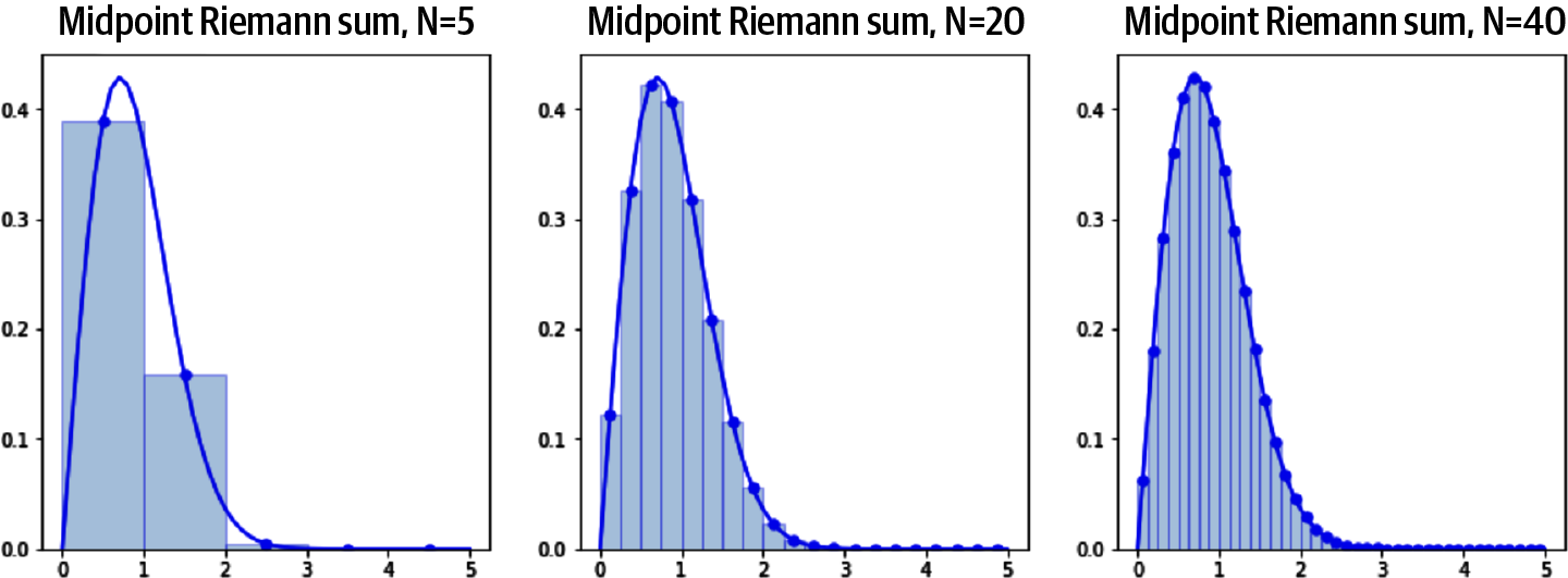
Figure 4-7. Formally, for reasonably well-behaved functions, as the number of rectangles goes to infinity, the error between the Riemann sum approximation and the true area under the curve goes to zero. This presents a trade-off when using Riemann sums to approximate continuous integrals.
Using the hyperparameter for the number of steps, we can approximate the integral for computing Integrated Gradients in the following way:
In the notebook discussing Integrated Gradients in the GitHub repository for this book, you can see how each component of this sum is computed directly in Python and TensorFlow in the integrated_gradients function. First, the ’s are created and the gradients are collected along the straight line path in batches. Here the argument num determines the number of steps to use in the integral approximation:
  # Generate alphas.
  alphas = tf.linspace(start=0.0, stop=1.0, num=m_steps+1)

  # Collect gradients.
  gradient_batches = []

  # Iterate alphas range and batch speed, efficiency, and scaling
  for alpha in tf.range(0, len(alphas), batch_size):
    from_ = alpha
    to = tf.minimum(from_ + batch_size, len(alphas))
    alpha_batch = alphas[from_:to]

    gradient_batch = one_batch(baseline, image, alpha_batch, target_class_idx)
    gradient_batches.append(gradient_batch)
Then those batch-wise gradients are combined into a single tensor and the integral approximation is computed, as shown in the following code. The number of gradients is controlled by the number of steps m_steps:
  # Concatenate path gradients.
  total_gradients = tf.concat(gradient_batches, axis=0)

  # Compute Integral approximation of all gradients.
  avg_gradients = integral_approximation(gradients=total_gradients)
Finally, we scale the approximation and return the integrated gradient results:
  # Scale Integrated Gradients with respect to input.
  integrated_gradients = (image - baseline) * avg_gradients
You can visualize these attributions and overlay them on the original image. The following code sums the absolute values of the Integrated Gradients across the color channels to produce an attribution mask:
  attributions = integrated_gradients(baseline=black_baseline,
                                      image=input_image,
                                      target_class_idx=target_class_idx,
                                      m_steps=m_steps)
  attribution_mask = tf.reduce_sum(tf.math.abs(attributions), axis=-1)
You can then overlay the attribution mask with the original image, as shown in Figure 4-8. See the notebook in the GitHub repository to see the full code for this example.

Figure 4-8. After computing feature attributions from the Integrated Gradients technique, overlaying the attribution mask over the original shows which parts of the image most contributed to the model’s class prediction.

Figure 4-9. The results of applying Integrated Gradients with a white baseline versus a black baseline are quite different for a predominantly white image, like a sulfur-crested cockatoo.
The code and discussion in this section show what’s really happening “under the hood” when implementing Integrated Gradients for model explainability. There are also more high-level libraries that can be leveraged and have easy-to-use implementations. In particular, the saliency library developed by the People + AI Research (PAIR) group at Google contains easy-to-use implementations of Integrated Gradients, its many variations, and other explainability techniques. See the notebook in the book’s GitHub repository to see how the saliency library can be used to find attribution masks via Integrated Gradients.
Improvements on Integrated Gradients
The method of Integrated Gradients is one of the most widely used and well-known gradient-based attribution techniques for explaining deep networks. However, for some input examples, this method can produce spurious or noisy pixel attributions that aren’t related to the model’s predicted class. This is partly due to the accumulation of noise from regions of correlated, high-magnitude gradients for irrelevant pixels that occur along the straight line path that is used when computing Integrated Gradients. This is also closely related to the choice of baseline that is used when computing Integrated Gradients for an image.
Various techniques have been introduced to address the problems that may arise when using Integrated Gradients. We’ll discuss two variations on the classic Integrated Gradients approach: Blur Integrated Gradients and Guided Integrated Gradients.
Blur Integrated Gradients (Blur-IG)
In the section “Choosing a Baseline,” you saw that when implementing Integrated Gradients, the choice of baseline is very important and can have significant effects on the resulting explanations. Blur Integrated Gradients (Blur-IG) specifically addresses the issues that arise with choosing a specific baseline. In short, Blur-IG removes the need to provide a baseline as a parameter and instead advocates to use the blurred input image as the baseline when implementing Integrated Gradients.
This is done by applying a Gaussian blur filter parameterized by its variance . We then compute the Integrated Gradients along the straight line path from this blurred image to the true, unblurred image. As increases, the image becomes more and more blurred, as shown in Figure 4-10. The maximum scale should be chosen so that the maximally blurred image is information-less, meaning the image is so blurred it wouldn’t be possible to classify what is in the image.

Figure 4-10. With no blur, the model predicts “goldfinch” with 97.5% confidence, but with , the model’s top prediction becomes “safety pin.”
The idea is that for different scale values of , different features are preserved or destroyed depending on the scale of the feature itself. The smaller the variation of the feature, the smaller the value of at which it is destroyed, as seen in the detail in the wing patterns of the goldfinch in Figure 4-10. When is less than 3, the black-and-white pattern on the wings is still recognizable. However, for larger values of , the wings and head are just a blur.
We can compare the saliency maps produced from using regular Integrated Gradients versus Blur Integrated Gradients (shown in Figure 4-11). Using the saliency library, this can be done in only a few lines of code:
# Construct the saliency object.
integrated_gradients = saliency.IntegratedGradients()
blur_ig = saliency.BlurIG()

# Baseline is a black image.
baseline = np.zeros(im.shape)

# Compute the IG mask and the Blur IG mask.
integrated_gradients_mask_3d = integrated_gradients.GetMask(
  im, call_model_function, call_model_args, x_steps=25, x_baseline=baseline,
  batch_size=20)
blur_ig_mask_3d = blur_ig.GetMask(
  im, call_model_function, call_model_args, batch_size=20)
In this code block, the call_model_function is a generic function that tells how to pass inputs to a given model and receive the outputs necessary to compute the saliency masks. It can be used with any ML framework. See the notebook on Integrated Gradients for the full code for this example. For this example of an image of an American goldfinch, Blur-IG produces much more convincing attributions than the vanilla Integrated Gradients.

Figure 4-11. The saliency map for Blur-IG does a much better job of recognizing the parts of the image that make up the goldfinch.
Guided Integrated Gradients (Guided IG)
Guided Integrated Gradients (Guided IG) attempts to improve upon Integrated Gradients by modifying the straight line path that is used in the implementation. Instead of using a straight line path from the baseline to the input image, Guided IG uses an adapted path to create saliency maps that are better aligned with the model’s prediction. Instead of moving pixel intensities in a fixed straight line direction from the baseline to the input, we make a choice at every step. More precisely, Guided IG moves in the direction where features (i.e., pixels) have the smallest absolute value of partial derivatives. As the intensity of the pixels becomes equal to those of the input image, they are ignored.
The idea is that the typical straight line path that is used by previous integrated gradient techniques we’ve discussed so far could potentially travel through points in the feature space where the gradient norm is large and not pointing in the direction of the integration path. As a result, the naive straight line path leads to noise and gradient accumulation in saturated regions that causes spurious pixels or regions to be attributed at too high of an importance when computing saliency maps. Guided IG avoids this problem by instead navigating along an adapted path in feature space, taking into account the geometry of the model surface in feature space. Figure 4-12 compares the result of applying vanilla Integrated Gradients with that of Guided Integrated Gradients. See the Integrated Gradients notebook in this book’s GitHub repository for the full code for this example.
For the example image in Figure 4-12, the saliency map for the Guided IG example seems to focus on the goldfinch in the image more than the saliency map for Integrated Gradients, but both methods don’t seem to do a particularly great job of producing convincing explanations. This may indicate that our model needs more training, or more data. Or maybe that both Integrated Gradients and Guided IG just aren’t well suited for this task or this dataset and another method would work better. There is no one-size-fits-all XAI technique. This is why it’s important to have a well-stocked toolkit of techniques that you can use when analyzing your model predictions.

Figure 4-12. The saliency map for the Guided IG example focuses on the goldfinch in the image more than the saliency map for Integrated Gradients, but both methods don’t seem to do a particularly great job of producing convincing explanations.
XRAI
Here’s what you need to know about XRAI:
XRAI is a region-based attribution method that builds upon Integrated Gradients.
XRAI determines regions of importance by segmenting the input image into like regions based on a similarity metric and then determines attribution scores for those like regions.
XRAI is a local explainability method that can be applied to any DNN-based model as long as there is a way to cluster the input features into segments through some similarity metric.
| Pros | Cons |
|---|---|
|
|
The saliency maps obtained from applying Integrated Gradients provide an easy-to-understand tool to visually see which pixels contribute most to a model’s prediction for a given image. XRAI builds upon the method of Integrated Gradients by joining pixels into regions. So instead of highlighting individual pixels that were most important, the saliency maps obtained by XRAI highlight pixel regions of interest in the image.
A key component and the first step of the XRAI algorithm is the segmentation of the image to determine those regions of interest. Image segmentation is a popular use case in computer vision that aims to partition an image into multiple regions that are conceptually similar, as illustrated in Figure 4-13.

Figure 4-13. Image segmentation is a process of assigning a class to each pixel in an image. Here are some examples from the Common Objects in Context (COCO) dataset.
Image segmentation is a well-studied problem in computer vision, and deep learning architectures like U-Net, Fast R-CNNs, and Mask R-CNNs have been developed to specifically address this challenge and can produce state-of-the-art results. One of the key steps of the XRAI algorithm uses an algorithm called Felzenszwalb’s algorithm to segment an input image into similar regions, much in the same way as a nearest neighbors clustering algorithm. The Felzenszwalb algorithm doesn’t rely on deep learning.3 Instead, it is a graph-based approach based on Kruskal’s minimum spanning tree algorithm and provides an incredibly efficient means to image segmentation. The key advantage of Felzenszwalb’s algorithm is that it captures the important nonlocal regions of an image that are globally relevant and, at the same time, is computationally efficient with time complexity where is the number of pixels.
The idea is to represent an image as a connected graph of vertices and edges where each pixel is a vertex in the graph and the edges connect neighboring pixels. The segmentation algorithm then iteratively tests the importance of each region and refines the graph partitions, coalescing smaller regions into larger segments until an optimal segmentation is found, resulting in a segmentation shown in Figure 4-14.

Figure 4-14. The Felzenszwalb segmentation algorithm realizes an image as a weighted undirected graph and then partitions the graph so that the variation across two different components is greater than the variation across either component individually.
The sensitivity to the within group and between group differences is handled by a threshold function. The strictness of this threshold is determined by the parameter . You can think of this as setting the scale of observation for the segmentation algorithm. Figure 4-15 shows the resulting image segmentations for various values of . These images were created using the segmentation package of the scikit-image library. The code for this example is available in this book’s GitHub repository. As you can see there, a larger value of causes a preference for larger components, while a smaller value of allows for smaller regions. It’s important to note that does not guarantee a minimum component size. Smaller components would still be allowed, they just require a stronger difference between neighboring components.

Figure 4-15. The parameter controls the threshold function for Felzenszwalb segmentation algorithm. A larger value of causes a preference for larger components while a smaller value of allows for smaller regions.
How XRAI Works
XRAI combines the output from applying Integrated Gradients to an input image with the image segmentation provided by Felzenszwalb’s algorithm described in the previous section. Intuitively, Integrated Gradients provides pixel-level attributions, so by aggregating these local feature attributions over the globally relevant segments produced from the image segmentation, XRAI is able to rank each segment and order the segments that contribute most to the given class prediction.
If one segment, for example the segment consisting of the body and crest of the cockatoo in Figure 4-14, contains a lot of pixels that are considered salient via Integrated Gradients, then that segment would also be ranked as highly salient via XRAI as well. However, a much smaller region, such as the segment representing the eye of the cockatoo, even if the pixels have high saliency measures according to the output from applying Integrated Gradients, XRAI would not rank that region as highly. This helps protect against individual pixels or small pixel segments that have spuriously high saliency from applying Integrated Gradients alone.
One thing to keep in mind, however, is the sensitivity of the segmentation result and how a certain choice of hyperparameters might bias the result. To address this, the image is segmented multiple times using different values (50, 100, 150, 250, 500, 1200) for the scale parameter . In addition, segments smaller than 20 pixels are ignored entirely. Since for a single parameter the union of segments gives the entire image, the union of all segments obtained from all the parameters yields an area equal to about six times the total image area and with multiple segments overlapping. Each of the regions from this oversegmentation is used when aggregating the lower-level attributions.
So, bringing it all together, when implementing XRAI, first the method of Integrated Gradients is applied using both a black and white baseline to determine pixel-level attributions, as shown in Figure 4-16. Concurrently, Felzenszwalb’s graph-based segmentation algorithm is applied multiple times using a range of scale parameter values for k = 50, 100, 150, 250, 500, 1200. This produces an oversegmentation of the original image. XRAI then aggregates the pixel-level attributions by summing the values from the integrated gradient output within each of the resulting segments and ranks each segment from most to least salient. The result is a heatmap that highlights the areas of the original image that contribute most strongly to the model’s class prediction. Overlaying this heatmap over the original image, we can see which regions most strongly contribute to the prediction of “sulfur-crested cockatoo.”

Figure 4-16. XRAI combines the results from the method of Integrated Gradients with the oversegmentation regions obtained from multiple applications of Felzenszwalb’s segmentation algorithm. The pixel-level attributions are then aggregated over the oversegmented regions and ranked to determine which regions are most salient for the model.
Implementing XRAI
XRAI is a post hoc explainability method and can be applied to any DNN-based model. Let’s look at an example of how to implement XRAI using the saliency library developed by the People + AI Research (PAIR) group at Google. In the following code block, we load a VGG-16 model pretrained on the ImageNet dataset and modify the outputs so that we can capture the model prediction m.output as well as one of the convolution block layers block5_conv3. The full code for this example can be found in the XRAI for Image Explainability notebook in this book’s GitHub repository:
m = tf.keras.applications.vgg16.VGG16(weights='imagenet', include_top=True)
conv_layer = m.get_layer('block5_conv3')
model = tf.keras.models.Model([m.inputs], [conv_layer.output, m.output])
To get the XRAI attributions, we construct a saliency object for XRAI and call the method GetMask passing in a few key arguments:
xrai_object = saliency.XRAI()
xrai_attributions = xrai_object.GetMask(image,
                                        call_model_function,
                                        call_model_args,
                                        batch_size=20)
The image argument is fairly self-explanatory: it’s the image on which we want to obtain the XRAI attributions passed in as a numpy array. Let’s discuss the other arguments: the call_model_function and call_model_args. The call_model_function is how we pass inputs to our model and receive the outputs necessary to compute a saliency mask. It calls the model so it expects input images. Any arguments needed when calling and running the model are handled by call_model_args. The last argument, expected_keys, tells the function the list of keys expected in the output. We’ll use the call_model_function defined in the following code, and we’ll either get back gradients with respect to the inputs or the gradients with respect to the intermediate convolution layer:
class_idx_str = 'class_idx_str'
def call_model_function(images, call_model_args=None, expected_keys=None):
    target_class_idx = call_model_args[class_idx_str]
    images = tf.convert_to_tensor(images)
    with tf.GradientTape() as tape:
        if expected_keys==[saliency.base.INPUT_OUTPUT_GRADIENTS]:
            tape.watch(images)
            _, output_layer = model(images)
            output_layer = output_layer[:,target_class_idx]
            gradients = np.array(tape.gradient(output_layer, images))
            return {saliency.base.INPUT_OUTPUT_GRADIENTS: gradients}
        else:
            conv_layer, output_layer = model(images)
            gradients = np.array(tape.gradient(output_layer, conv_layer))
            return {saliency.base.CONVOLUTION_LAYER_VALUES: conv_layer,
                    saliency.base.CONVOLUTION_OUTPUT_GRADIENTS: gradients}
You may recall that when implementing Integrated Gradients, one hyperparameter you could adjust is the number of steps used to compute the line integral. Since XRAI relies on the output from Integrated Gradients, you may be wondering where and how you adjust that hyperparameter for XRAI. In the saliency library, those kinds of hyperparameters are controlled with a subclass called XRAIParameters. The default number of steps is set to 100. To change the number of steps to 200, you simply create an XRAIParameters object and pass it to the GetMask function as well:
xrai_params = saliency.XRAIParameters()
xrai_params.steps = 200

xrai_attributions_fast = xrai_object.GetMask(im,
                                             call_model_function,
                                             call_model_args,
                                             extra_parameters=xrai_params,
                                             batch_size=20)
Finally, we can plot the xrai_attributions object returned from calling GetMask to obtain a heatmap of attributions for the image, as shown in Figure 4-17.
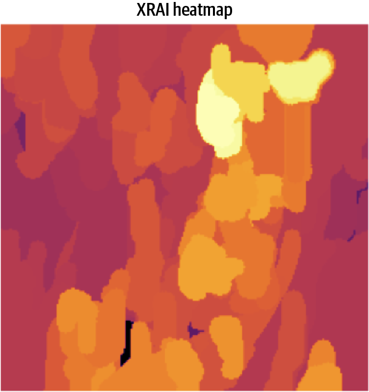
Figure 4-17. XRAI produces a heatmap of attributions for a given input image. For this image of a sulfur-crested cockatoo, the more relevant regions correspond to the body of the bird, its beak, and its distinct crest.
In order to see which regions of the original image were most salient, the following code focuses only on the most salient 30% and creates a mask filter overlaid on the original image. This results in Figure 4-18:
mask = xrai_attributions > np.percentile(xrai_attributions, 60)
im_mask = np.array(im_orig)
im_mask[~mask] = 0
ShowImage(im_mask, title='Top 30%', ax=P.subplot(ROWS, COLS, 3))

Figure 4-18. Filtering the XRAI attributions, we can overlay the heatmap on the original image to highlight only the most salient regions.
Grad-CAM
Here’s what you need to know about Grad-CAM:
Grad-CAM is short for Gradient-weighted Class Activation Mapping. Grad-CAM was one of the first explainability techniques; it generalizes CAM that could only be used for certain model architectures.
Grad-CAM works by examining the gradient information flowing through the last (or any) convolution layer of the network.
It produces a localization heatmap highlighting the regions in an image most influential for predicting a given class label.
| Pros | Cons |
|---|---|
|
|
Grad-CAM is one of the original explainability techniques developed for image models and can be applied to any CNN-based network. Grad-CAM is a post hoc explanation technique and doesn’t require any architecture changes or retraining. Instead, Grad-CAM accesses the internal convolutions layers of the model to determine regions that are most influential for the model’s predictions. Because Grad-CAM only relies on forward passes through the model, with no backpropagation, it is also computationally efficient.
How Grad-CAM Works
To understand how Grad-CAM works, let’s first start with what Class Activation Map (CAM) is and how it works, since Grad-CAM is essentially a generalization of CAM. Typically, when building an image model, your model architecture is likely to consist of a stack of convolutional and pooling layers. For example, think about the classic VGG-16 model architecture shown in Figure 4-19. There are five convolution plus pooling blocks that act as feature extractors, followed by three fully connected layers (FC) before the final softmax prediction layer. CAM is a localization map of the image that is computed as a weighted activation map. This is done by taking a weighted sum of the activation maps of the final convolution layer in the model.
More precisely, and to illustrate with an example, suppose we take the final convolution layer (just before the last pooling layer) of the VGG-16 model in Figure 4-19 trained on the ImageNet dataset. The dimension of this final convolution layer is 7×7×512. So, there are 512 feature maps mapping to 1,000 class labels; that is, the labels corresponding to ImageNet.

Figure 4-19. VGG-16 consists of blocks of convolution and pooling layers. CAM is a weighted activation map applied to the final convolution layer.
Each feature map is indexed by and representing the width and height of the convolution layer (in this case ). Notationally, denotes the activation at location of the feature map . Those feature maps are then pooled using global average pooling and CAM computes a final score for each class by taking a weighted sum of the pooled feature maps, where the weights are given by the weights connecting the -th feature map with the -th class:
If you then take the gradient of , that is, the score for class , with respect to the feature maps, you can separate out the weight term , so that (after a bit of math4) you get:
This weight value is almost exactly the same as the neuron importance weight that is used in Grad-CAM! For Grad-CAM, you also pull out the activations from the final convolution layer and compute the gradient of the class score with respect to these . In some sense, these gradients capture the information flowing through the last convolution layer; you want to use this to assign importance values to each neuron for a particular class . This importance weight is computed (similarly to CAM) as:
The last step of Grad-CAM is to then take a weighted combination of the activation maps using these as weights and apply a ReLU to that linear combination, as shown in Figure 4-20. So,
You use a ReLU here because we only care about the pixels whose intensity should be increased in order to increase the class score . Remember ReLU maps negative values to zero, so by applying ReLU after the weighted sum we only capture the positive influence on the class score. Because the shape of is the same shape as the final convolution layer; it produces a coarse heatmap that can then be overlaid on the original image to indicate which regions were most influential in the model predicting class . Also, due to the averaging and pooling of these feature maps, Grad-CAM works best at representing regions of influence in the image rather than exact pixels. An overview of the Grad-CAM process is shown in Figure 4-20.

Figure 4-20. An overview of Grad-CAM. The final activation maps are used to compute a weighted sum that is then passed through a ReLU layer.
The coarse heatmap created by Grad-CAM is problematic and can generate misleading results. Because the heatmap has the same dimensions as the final convolutional feature maps , it is usually upsampled to fit the shape of the original image. For example, the last convolutional layer of VGG-16 is 7×7×512, so the heatmap determined from the weighted sum of the activation maps will have dimension 7×7, which then has to be upsampled to overlay on the original image that has shape 224×224. This upsampling has the strong potential for causing misleading results, particularly if your dataset consists of large images whose shape is much larger than the internal activation map or contains image patterns and artifacts that are not properly sampled by a convolution.
You may be wondering how exactly Grad-CAM improves upon CAM, especially if they are essentially using the same importance weights. The advantage of Grad-CAM is that the construction for CAM is very limiting. It requires feature maps to directly precede softmax layers. So, CAM only works for certain kinds of CNN model architectures, i.e., ones that have their final layers to be a convolution feature mapped to a global average pooling layer mapped to a softmax prediction layer. The problem is that this may not be architecture with best performance. By taking a gradient and rearranging terms, Grad-CAM is able to generalize CAM and works just as well for a wide range of architectures for other image-based tasks, like image captioning or visual question answering.
In the description of Grad-CAM, we only discussed taking the CAM from the final convolution layer. As you may have already guessed, the technique we described is quite general and can be used to explain activations for any layer of the deep neural network.
Implementing Grad-CAM
The Grad-CAM algorithm outlined in Figure 4-20 is fairly straightforward and can be implemented directly by hand, assuming you have access to the internal layers of your CNN model. However, there is an easy-to-use implementation available from the saliency library. Let’s see how it works with an example. You start by creating a TensorFlow model. In the following code block, we load a pretrained VGG-16 model architecture that has been trained on the ImageNet dataset. We also select the penultimate convolution layer block5_3 that we’ll use to obtain the activation maps. Note that when we build the actual model it returns both the convolution layer output and the VGG-16 outputs, so we can still make predictions. For the full code for this example, see the Grad-CAM notebook in the GitHub repository for this book:
vgg16 = tf.keras.applications.vgg16.VGG16(
    weights='imagenet', include_top=True)
conv_layer = m.get_layer('block5_conv3')
model = tf.keras.models.Model(
    [vgg16.inputs], [conv_layer.output, vgg16.output])
To apply Grad-CAM, you then construct a saliency object, calling the Grad-CAM method and then apply GetMask passing the example image, and the call_model_function. The following code block shows how this is done. The call_model_function interfaces with a model to return the convolution layer information and the gradients of the model. This returns a Grad-CAM mask that can be used to plot a heatmap indicating influential regions in the image:
# Construct the saliency object. This alone doesn't do anything.
grad_cam = saliency.GradCam()

# Compute the Grad-CAM mask.
grad_cam_mask_3d = grad_cam.GetMask(im, call_model_function,
call_model_args)
Historically, Grad-CAM is an important technique. It was one of the first techniques to leverage the internal convolution layers of a CNN model to derive explanations for model prediction. However, you should take caution when implementing and interpreting the results from Grad-CAM. Because of the upsampling and smoothing step from the convolution layer, some regions of the heatmap may seem important when in fact they were not influential for the model at all. There have been improvements to address these concerns (see the next section, “Improving Grad-CAM,” and the later section “Guided Grad-CAM”), but the results should be viewed critically and in comparison with other techniques.
Improving Grad-CAM
After publication of the original paper in 2017,5 it was discovered that Grad-CAM could inaccurately attribute model attention to regions of the image that were not actually influential in the prediction. Grad-CAM applies a natural smoothing, or interpolation, to its original heatmaps in enlarging them to the size of the original dimensions of the input image. Figure 4-21 shows an example of what the Grad-CAM output looks like with and without smoothing.
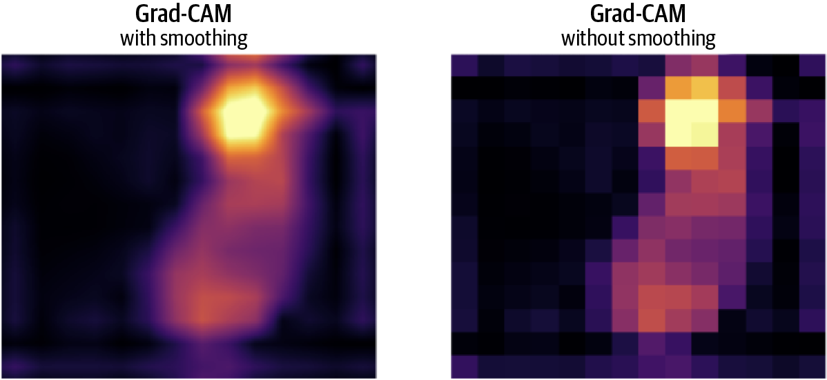
Figure 4-21. Grad-CAM upsamples from the feature map size to the size of the original image and applies a natural smoothing. This can cause misleading results and inaccurately attribute model attention to regions that weren’t influential.
The smoothing results in a more visually pleasing image, with seamless changes in the colors of the heatmap, but can also be very misleading. Since the original region was focused on a much smaller image size, we can’t say that the pixels that were lost would have had the same influence on the model as those remaining around it.6 In response, researchers developed Grad-CAM++ and HiResCAM to address these issues. Figure 4-22 shows an example of how the outputs of Grad-CAM and Grad-CAM++ differ. These newer techniques helped to address these concerns and can produce more accurate attribution maps. However, even with the regional inaccuracy fixed, Grad-CAM remains a flawed technique due to how it upsamples from the original size of the feature maps to the size of the input image.
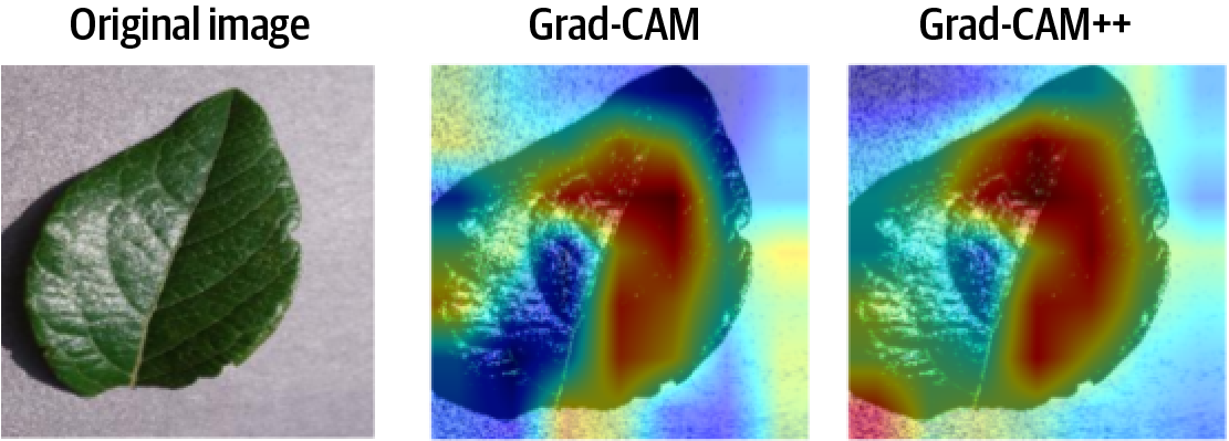
Figure 4-22. A heatmap from applying Grad-CAM and Grad-CAM++ for the classification of a healthy blueberry leaf. In the Grad-CAM image, the heatmap is most attentive in the center of the leaf but also highlights some influence from the background. For Grad-CAM++, the activated pixels are more evenly distributed throughout the leaf, although a highly influential region is still attributed to the background in the lower left. (Print readers can see the color image at https://oreil.ly/xai-fig-4-22.)
LIME
Here’s what you need to know about LIME:
LIME stands for local interpretable model-agnostic explanations. It is a post hoc, perturbation-based explainability technique.
LIME can be used for regression or classification models, though in practice LIME is used primarily for classification models.
LIME works by changing regions of an image, turning them on or off and rerunning inferences to see which regions are most influential to the model’s prediction.
LIME uses an inherently interpretable model to measure influence or importance of input features.
| Pros | Cons |
|---|---|
|
|
Due to its age, LIME is one of the more popular explainability techniques. It can also be used for tabular and text data, and the algorithm is similar for each of these data modalities albeit with some modifications. We discuss the details of implementing LIME with images here because it gives a nice visual intuition of how LIME works in general (see Chapter 5 for a discussion of how LIME works with text).
How LIME Works
LIME is a post hoc, model-agnostic, perturbation-based explainability technique. That means it can be applied to any machine learning model (e.g., neural networks, SVM, random forest, etc.) and is applied after the model has been trained. In essence, LIME treats the trained model like an API, taking an example instance and producing a prediction value. To explain why the model makes a certain prediction for a given input instance, the LIME algorithm works by passing lots and lots of slightly perturbed examples of the original input to the model and then measures how the model predictions change with these small input changes. The perturbations occur at the feature level of the input instance; i.e., images, pixels, and pixel regions are modified to create a new perturbed input. In this way, those pixels or pixel regions that most influence the model’s prediction are highlighted as being more or less influential to the model’s predicted output for the given input instance.
To go into a little more detail, let’s further explain two of the key components of implementing LIME: first, how to generate a perturbation of an image and second, what it means to measure how the model prediction changes on these perturbations.
For a given prediction, the input image is subdivided into interpretable components, or regions, of the image. LIME segments the image into regions called superpixels. A superpixel is a similarity-based grouping of the individual pixels of an image into similar components (see the discussion of Felzenszwalb’s algorithm in the earlier section “XRAI”). For example, Figure 4-23 shows how the image of the sulfur-crested cockatoo can be segmented into superpixels. The superpixel regions represent the interpretable components of the image.

Figure 4-23. When implementing LIME, the original image is segmented into superpixel regions that represent the interpretable components of the image.
The superpixel regions in Figure 4-23 were created using the quickshift segmentation algorithm from the scikit-image library. This is the default segmentation algorithm used in the widely used, open source Python package LIME (see the next section, “Implementing LIME”), although other segmentation functions could be used. Quickshift is based on an approximation of kernelized mean-shift and computes hierarchical segmentation at multiple scales simultaneously. Quickshift has two main parameters: the parameter sigma determines the scale of the local density approximation, and max_dist determines the level of the hierarchical segmentation. There is also a parameter ratio that controls the ratio between the distance in color space and the distance in image space when comparing the similarity of two pixels. The following code produces the segmentation in Figure 4-23. See the LIME notebook in the GitHub repository for this book for the full code example:
from skimage.segmentation import quickshift

segments = quickshift(im_orig, kernel_size=4,
                      max_dist=200, ratio=0.2)
LIME then perturbs these interpretable components by changing the values of the pixels in each superpixel region to be gray. This creates multiple new variations, or perturbations, of the input image. Each of these new perturbed instances is then given to the model to generate new prediction values for the class that was originally predicted. For example, in Figure 4-24 the original image is modified by graying out certain superpixel regions. Those perturbed examples are then passed to the trained model (in this case a deep neural network), and the model returns the probability that the image contains a sulfur-crested cockatoo. These new predictions create a dataset that is used to train LIME’s linear model to determine how much each interpretable component contributes to the original prediction.
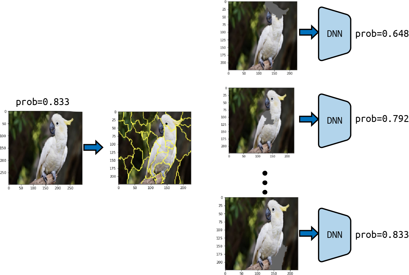
Figure 4-24. The model’s confidence in the predicted class “sulfur-crested cockatoo” for the original image is 0.833. As certain superpixels are removed (by graying out the region), the model’s top class prediction changes. For regions that are influential, the change is larger than for regions that are less important.
In the LIME implementation, superpixels are turned “on” or “off” by changing the pixel values of a segment to gray. This creates a collection of perturbed images that are passed to the model for prediction. It is also possible to instead change the superpixel regions to the mean of the individual pixel values in the superpixel region, as shown in Figure 4-25.

Figure 4-25. It is also possible to perturb images by setting the values of superpixel regions to be the average of the individual pixel regions in the image.
Let’s now discuss how LIME quantitatively measures the contributions of the superpixel feature inputs. This is done by training a smaller, interpretable model to provide explanations for the original model. This smaller model can be anything, but the important aspect is that it is inherently interpretable. In the original paper,7 the authors use the example of a linear model. Linear models are inherently interpretable because the weights of each feature directly indicate the importance of that feature for the model’s prediction.
This interpretable, linear model is then trained on a dataset consisting of the perturbed examples and the original model’s predictions, as shown in Figure 4-24. These perturbations are really just simple binary representations of the image indicating the “presence” or “absence” of each superpixel region. Since we care about the perturbations that are closest to the original image, those examples with the most superpixels present are weighted more than examples that have more superpixels absent. This proximity can be measured using any distance metric for images. The idea is that even though your trained model might be highly complex, for example a deep neural network or an SVM, the locally weighted, linear model can capture the local behavior at a given input instance. The more sensitive the complex model is to a given input feature, the more of an influence that feature will have on the linear, interpretable model as well.
Implementing LIME
There is a nice, easy-to-use Python package for applying LIME to tabular, image, and text classifiers that works for any classifier with at least two label classes. As an example, let’s see how to implement LIME on the Inception v3 image classification model. The following code shows how to load the image in TensorFlow and make a prediction on an image. Note that when we load the incepton model, we specify include_top=True to get the final prediction layer of the model and we set weights='imagenet' to get the weights pretrained on the ImageNet dataset:
inception = tf.keras.applications.InceptionV3(
    include_top=True, weights='imagenet')
model = tf.keras.models.Model(inception.inputs, inception.output)
Now, given an image, we can create explanations for the Inception model’s prediction by creating a LimeImageExplainer object and then calling the explain_instance method. The following code block shows how to do this:
explainer = lime_image.LimeImageExplainer()
explanation = explainer.explain_instance(image.astype('double'),
                                         inception.predict,
                                         top_labels=20,
                                         hide_color=0,
                                         num_features=5)
Most of the parameters in this code block are self-explanatory. The last two, however, are worth mentioning. Firstly, the parameter hide_color indicates that we’ll turn off superpixel regions by replacing them with gray pixels. The parameter num_features indicates how many features to use in the explanation. Fewer features lead to more simple, understandable explanations. However, for more complex models it may be necessary to keep this value large (the default is num_features=100000).
To visualize the explanations for this example, we then call get_image_and_mask on the resulting explanation. This is shown in the following code block; see the LIME notebook in the book repository for the full code for this example:
temp, mask = explanation.get_image_and_mask(explanation.top_labels[0],
                                            positive_only=True,
                                            num_features=20,
                                            hide_rest=True)
plt.imshow(mark_boundaries(temp, mask))
plt.show()
The result is shown in Figure 4-26, which highlights the superpixel regions that most positively contributed to the prediction “sulfur-crested cockatoo.”

Figure 4-26. LIME uses a linear model trained on perturbations of the original input image to determine which superpixel regions were most influential for the complex model’s prediction.
It is also possible to see which superpixel regions provide a negative contribution as well. To do this, set positive_only to False. This produces the output image as shown in Figure 4-27. The regions that positively contribute to the prediction are in green, while the regions that negatively influence the prediction are in red.

Figure 4-27. A LIME explanation. Regions that influenced the model are shown as a heatmap, with more influential regions having a deeper color, where green contributed positively to the classification, and red contributed negatively. (Print readers can see the color image at https://oreil.ly/xai-fig-4-27.)
This results in a segmented map of the image that is weighted according to how strongly that region influenced the model’s prediction. Unlike Shapley values, there are no bounds or guarantees on the values of the region. For example, LIME could conceivably weight multiple regions as highly influential.
Unfortunately, LIME’s elegance in generating weightings by turning regions of the image on and off is also its downfall. Since the perturbed images remove entire areas from the prediction, it effectively is shifting the model’s attention to what remains visible in the image. In effect, LIME is asking the model not to do a “limited” prediction of the original image, but to look at an entirely new image. However, by not holistically perturbing the entire image, like Integrated Gradients, it is possible that learned concepts in the model are no longer activated. We are asking the model to tell us how it would predict the image by looking at how predictions change only with respect to one feature value and assuming that comparing across different features will result in something akin to how the model made its original prediction. This can sometimes lead to nonsensical explanations, as shown in Figure 4-28.

Figure 4-28. An example of how LIME’s perturbation approach can lead to what seem to be nonsensical explanations. In the image of the goldfinch, there is a large portion of the background (nearly as much as the bird itself) contributing to the prediction. In the image of the cockatoo, we also see the background having a positive influence on the model, while parts of the bird have a negative influence as well. (Print readers can see the color image at https://oreil.ly/xai-fig-4-28.)
One way to address this problem is to adjust the parameters of the segmentation step: with more fine-grained segments, the less likely those superpixels will contribute to the image prediction. Ultimately, as with all implementations, it’s important to be aware of this artifact both when implementing LIME as a technique and when interpreting the results.
As a further example of this, we used LIME on a nonnatural dataset, the PlantVillage dataset, which contains images of plant leaves with disease and tries to predict the type of disease. These images feature a combination of a very natural image (plant leaves) within a much more structured environment (interior lighting, monochrome background). The model used, Schuler, was highly accurate, with an overall prediction accuracy of 99.8%. We also compared the LIME explanations to another, slightly less accurate model, Yosuke.

Figure 4-29. Examples of using LIME to explain the classifications between two different models. (Print readers can see the color image at https://oreil.ly/xai-fig-4-29.)
As you can see in the examples in Figure 4-29, LIME has determined that the backgrounds of the images are some of the most influential areas in the prediction. Given that the background is the same for all images in the dataset, this seems highly unlikely to be what is the cause for predictions!
Guided Backpropagation and Guided Grad-CAM
Here’s what you need to know about Guided Backprop (often abbreviated this way) and Guided Grad-CAM:
Guided Backprop builds on DeConvNets, which examines the interior layers of a convolution network.
Guided Backprop corresponds to the gradient explanation, setting negative gradient entries to zero while backpropagating through a ReLU unit.
Guided Grad-CAM combines the output of Grad-CAM and Guided Backprop through element-wise product to produce sharper visualizations in the saliency maps.
| Pros | Cons |
|---|---|
|
|
a Julius Adebayo et al., “Sanity Checks for Saliency Maps,” arXiv, 2020, https://arxiv.org/pdf/1810.03292.pdf. | |
As we’ve seen throughout this chapter, the gradients of a neural network are a useful tool for measuring how information propagates through a model to eventually create a prediction. The idea is that by measuring the gradients through backpropagation, you can highlight those pixels or pixel regions that contributed most to the model’s decision. Despite this intuitive approach, in practice the results of saliency maps that rely solely on gradient information can be very noisy and difficult to interpret. Guided Backprop also relies on model gradients to produce a saliency map but modifies the backpropagation step slightly in how it handles the ReLU nonlinearities.
Guided Backprop and DeConvNets
The technique of Guided Backprop is closely related to an earlier explainability method called DeConvNets. We’ll start by describing how DeConvNets work first, then see how Guided Backprop improves upon that approach. As the name suggests, DeConvNets are built upon deconvolution layers, also known as transposed convolutions. You can think of a deconvolution as an inverse of a convolution layer, its job is to “undo” the operation of a convolution layer. Figure 4-30 shows the typical architecture of a DeConvNet.

Figure 4-30. A typical deconvolution network with a VGG-16 backbone. The DeConvNet architecture starts with the usual convolution and max pooling layers, followed by deconvolution and unpooling layers.
As you can see from the figure, the DeConvNet architecture starts with a usual convolution network. Each convolutional layer passes a kernel over the input channels and calculates an output based on the weights of the filter. The size of the output of a convolution layer is determined by the kernel size, the padding, and the stride. For example, if you have an input tensor with shape (5,5) and a convolution layer with kernel size 3×3, stride set to 2, and zero padding, the output will be a tensor of shape (2,2), as shown on the left in Figure 4-31. The nine values in the base (5,5) tensor are aggregated as a linear combination to produce the single value in the resulting (2,2) tensor. If the input has multiple channels, the convolution is applied to each channel.
The second part of the DeConvNet is the deconvolution (or transposed convolution) layers. DeConvNets are similar to convolutional networks but work in reverse (reversing filters, reversing pooling, etc.) so that they reconstruct the spatial resolution of the original input tensor. There are two components to the DeConvNet: the deconvolution and the unpooling layers. We’ll discuss how the deconvolution layers work first. The deconvolution also uses a convolution filter but enforces additional padding both outside and within the input values to reconstruct the tensor with larger shape. For the convolution step we just described, the deconvolution maps the (2,2) tensor back to a tensor of shape (5,5), as shown in the image on the right in Figure 4-31. The deconvolution filter has size 3×3. In order to upsample the (2,2) tensor to a tensor of shape (5,5), we add additional padding on the outside and between input values (in red in Figure 4-31).
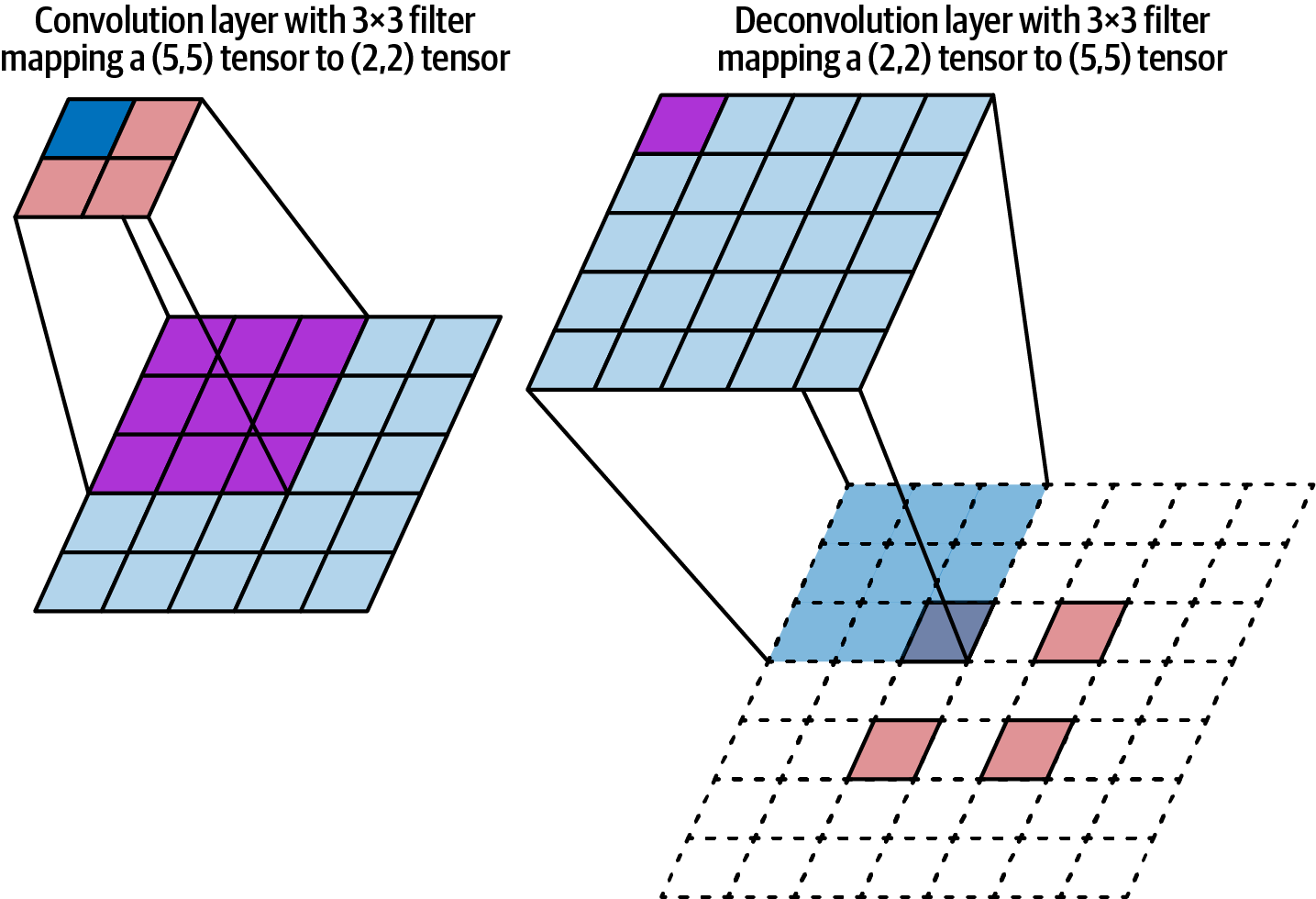
Figure 4-31. A deconvolution layer, shown on the right, reconstructs the original spatial resolution of the input to a convolution layer, shown on the left.
The next component of the DeConvNet to discuss are the unpooling layers. The max pooling layers of a convolution network pass a filter over the input and record only the maximum of all values in the filter as the output. By nature, max aggregation loses a lot of information. To perform unpooling, we need to remember the position where the maximum value occurred in the original max pooling filter. These locations are called switch variables. When performing unpooling, we place the max value from max pooling back in its original position and leave the rest of the values in the filter as zero, as shown in Figure 4-32.

Figure 4-32. When reversing a max pooling layer using “unpooling,” the switch variable keeps track of where the max value was located.
The idea of using DeConvNets as an explainability method is to visualize the internal activation layers of a trained CNN by “undoing” the convolution blocks of a CNN using deconvolution layers block by block. Ultimately, the DeConvNet maps the filter of an activation layer back to the original image space, allowing you to find patterns in the images that caused that given filter activation to be high.
Applying a convolution and max pooling causes some information of the original input tensor to be lost. This is because the convolution filter is aggregating values and the max pooling returns only one value from the entire filter, dropping the rest. The deconvolution reverses the convolutions step but it is an imperfect reconstruction of the original tensor.
The method of Guided Backpropagation is similar to DeConvNets. The difference is in how Guided Backprop handles backpropagation of the gradient through the ReLU activation functions. A DeConvNet only backpropagates positive signals; that is, it sets all negative signals from the backward pass to zero. The idea is that we are only interested in what image features an activation layer detects, not the rest, so we only focus on positive values. This is done by multiplying the backward pass by a binary mask so that only positive values are preserved. In Guided Backprop, you also restrict just the positive values of the input to a layer. So, a binary mask is applied both for the backward pass and the forward pass. This means there are more zero values in the final output, but it leads to sharper saliency maps and more fine-grained visualizations.
Here the name “Guided” indicates that this method uses information from the forward pass in addition to the backward pass to create a saliency map. The forward pass information helps to guide the deconvolution. This is similar in spirit to how Guided Integrated Gradients differs from vanilla Integrated Gradients in that it uses information about the baseline and the input to guide the path when computing a line integral.
Guided Grad-CAM
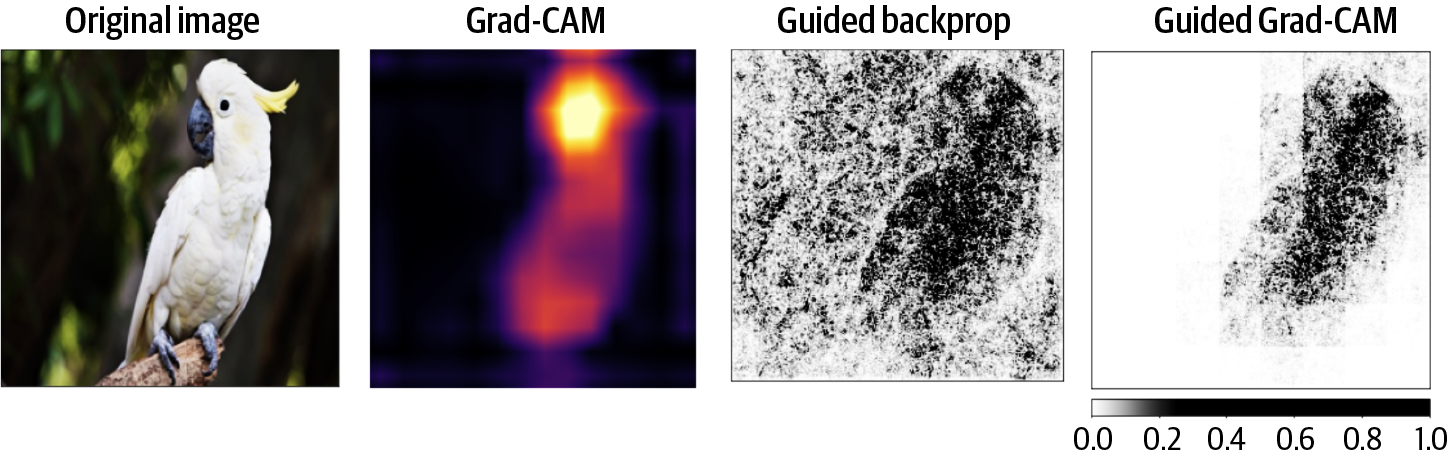
Guided Grad-CAM combines the best of both Grad-CAM and Guided Backprop. As we saw in the section on Grad-CAM, one of the problems with Grad-CAM was that the coarse heatmap produced from the activation layers must be upsampled so that it can be compared against the original input image. This upsampling and the subsequent smoothing leads to a lower-resolution heatmap. The original authors of Grad-CAM proposed Guided Grad-CAM as a way to combine the high-resolution output from Guided Backprop with the class-specific gradient information obtained from Grad-CAM alone. This doesn’t alleviate all of the concerns with Grad-CAM since it still relies on the output of the Grad-CAM technique, which has some fundamental concerns (see “Grad-CAM” for more in-depth discussion on this), but it is an improvement. Guided Grad-CAM combines Grad-CAM and Guided Backprop by taking an element-wise product of both outputs, as shown in Figure 4-33.

Figure 4-33. Guided Grad-CAM combines the output of Grad-CAM and Guided Backpropagation by taking the element-wise product. This produces a visualization.
Both Guided Backprop and Guided Grad-CAM have easy-to-use implementations available in the Captum library. Let’s look at an example to see how these techniques are implemented in code. Captum is built on PyTorch, so let’s start by loading an Inception v3 model that has been pretrained on the ImageNet dataset. This is done in the following code block (see the Guided Backprop notebook in this book’s GitHub repository for the full code for these examples):
import torch
model = torch.hub.load('pytorch/vision:v0.10.0',
                       'inception_v3',
                       pretrained=True)
model.eval()
In this code block, model.eval() tells PyTorch that we’re using the model for inference (i.e., evaluation), not for training. To create attributions using Guided Backprop, only a couple lines of code are required. First, we create our GuidedBackProp attribution object by passing the Inception model we previously created, then we call the attribute method passing the input example (as a batch of one) and the target class ID that we want to create explanations for. Here we set target=top5_catid[0] to use the top predicted class for the given input image, as shown in the following code block:
gbp = GuidedBackprop(model)
# Computes Guided Backprop attribution scores for class 89 (cockatoo)
gbp_attribution = gbp.attribute(input_batch, target=top5_catid[0])
This returns an attribution mask that we can then visualize using Captum’s visualization library. The result is shown in Figure 4-34.
You can implement Grad-CAM using the Captum library in a very similar way. Remember, Grad-CAM works by creating a coarse heatmap from the internal activation layers of the CNN model. These internal activations can be taken from any of the convolution layers of the model. So, when implementing Grad-CAM you specify which convolution layer to use for creating the heatmap. Similarly, for Guided Grad-CAM you specify which layer of the model as well. This is shown in the following code block. When creating the GuidedGradCam object, we pass the model as well as the layer model.Mixed_7c; this is the last convolution layer of the Inception v3 model:
from captum.attr import GuidedGradCam

guided_gc = GuidedGradCam(model, model.Mixed_7c)
ggc_attribution = guided_gc.attribute(
input_batch, target=top5_catid[0])
Once we have the attributions, we can visualize the result using Captum’s visualization library as before. See the Guided Backprop notebook in the GitHub repository for the full code for this example.
Summary
Computer vision models have critical applications in a wide range of contexts, from healthcare and security to manufacturing and agriculture. Explainability is essential for debugging a model’s predictions and assuring a model isn’t learning spurious correlations in the data. In this chapter, we looked into various explainability techniques that are used when working with image data.
Loosely speaking, explanation and attribution methods for computer vision models can be fit into a few broad categories: backpropagation methods, perturbation methods, methods that leverage the internal state of the model, and methods that combine different approaches. The explainability techniques we discussed in this chapter are representative examples of these categories, and each method has their own pros and cons.
Integrated Gradients and its many variations fall in the category of back-propagation techniques. XRAI combines Integrated Gradients with segmentation-based masking to determine regions of the image that are most important in the model’s prediction. By oversegmenting the image and aggregating smaller regions of importance into larger regions based on attribution scores, this produces more human-relatable saliency maps instead of pixel-level attributions obtained via Integrated Gradients alone. Methods like Grad-CAM and Grad-CAM++ also rely on gradients, but they leverage the internal state of the model. More specifically, Grad-CAM uses the class-activation maps of the internal convolutional layers of the model to create a heatmap of influential regions for an input image.
LIME is a model-agnostic approach that treats the model as opaque and determines pixels that are relevant to the model’s prediction by perturbing input pixel values. These methods use gradients of the model to create saliency maps (also called sensitivity maps or pixel attribution maps) to represent regions of an image that are particularly important for the model’s final classification. Lastly, we discussed Guided Backpropagation and Guided Grad-CAM, which combine different approaches. Guided Grad-CAM combines Guided Backprop and Grad-CAM using an element-wise product, getting the best of both methods, and addresses some of the problems that arise when using Grad-CAM.
In the next chapter, we’ll look into explainability techniques that are commonly used for text-based models and how some of the techniques that we’ve already seen can be adapted to work in the domain of natural language.
1 This is analogous to many loss-based functions for training DNNs that measure the gradient and performance change of the model in the loss space.
2 Mukun Sundararajan et al., “Axiomatic Attribution for Deep Networks,” Proceedings of the 34th International Conference on Machine Learning, PMLR 70 (2017).
3 Pedro F. Felzenszwalb and Daniel P. Huttenlocher, “Efficient Graph-Based Image Segmentation,” International Journal of Computer Vision 59.2 (2004): 167–81.
4 Ramprasaath R. Selvaraju et al., “Grad-CAM: Visual Explanations from Deep Networks via Gradient-Based Localization,” Computer Vision Foundation, https://oreil.ly/cU9sG.
5 The Grad-CAM paper was revised and updated in 2019.
6 Defenders of Grad-CAM claim that this upscaling is acceptable because it mirrors the downsampling performed by the model’s CNNs, but this argument does not have any strong theoretical grounding or evaluations to substantiate this claim.
7 Marco Tulio Ribeiro et al., “‘Why Should I Trust You?’ Explaining the Predictions of Any Classifier,” Proceedings of the 22nd SIGKDD International Conference on Knowledge Discovery and Data Mining (August 2016).
Get Explainable AI for Practitioners now with the O’Reilly learning platform.
O’Reilly members experience books, live events, courses curated by job role, and more from O’Reilly and nearly 200 top publishers.

