Feedback Control for Computer Systems

Chapter 23. Poles and Zeros

An important advantage of the “transfer function technology” is that we do not need to evaluate the entire transfer function to obtain information about a system’s dynamics. Instead, it is sufficient to merely know the locations of the transfer function’s poles and zeros—that is, the locations where the transfer function diverges or vanishes (respectively) to gain substantial insight into the dynamic behavior.

Structure of a Transfer Function

By construction, the transfer functions for feedback systems tend to be proper rational functions—that is fractions of one polynomial in s over another polynomial in s:

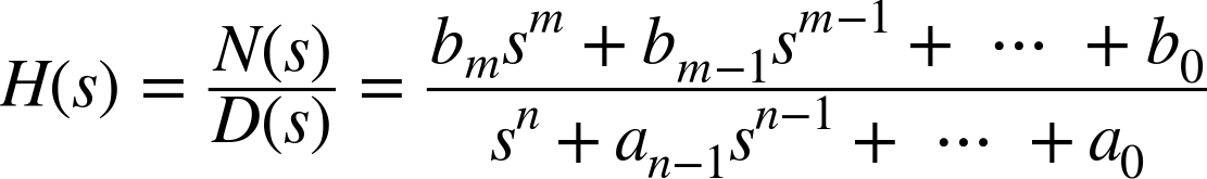
This fact is a consequence of the way transfer functions arise as solutions of linear differential equations with constant coefficients via Laplace transforms. (If the dynamics include time delays, then additional factors of the form e^–sT occur in the transfer function—more on this issue later in this chapter.)

The degree of a polynomial is the power of its highest term. In the preceding formula, the numerator is of degree m, and the denominator is of degree n. A transfer function is called strictly proper if it tends to 0 for large s, and it is called proper if it tends to a finite value as s approaches infinity. For transfer functions that are strictly rational functions, this means that for a transfer function to be strictly proper, the degree of the ...