Getting Started with SQL

Chapter 4. SELECT

When working with databases and SQL, the most common task is to request data from one or more tables and display it. The SELECT statement accomplishes this. But the SELECT can do far more than simply retrieve and display data. As we will learn in coming chapters, we can transform this data in meaningful ways and build powerful summaries from millions of records.

But first, we will learn how to SELECT columns from a single table as well as compose expressions in them.

Retrieving Data with SQL

If you have not done so already, click on Tools→Open SQL Editor in the top menu, and make sure the rexon_metals database is open, as mentioned in the previous chapter. Your SQLiteStudio workspace should look something like Figure 4-1. Notice that the SQL workspace is now divided into two panes, a SQL Editor pane and a Query Results pane.

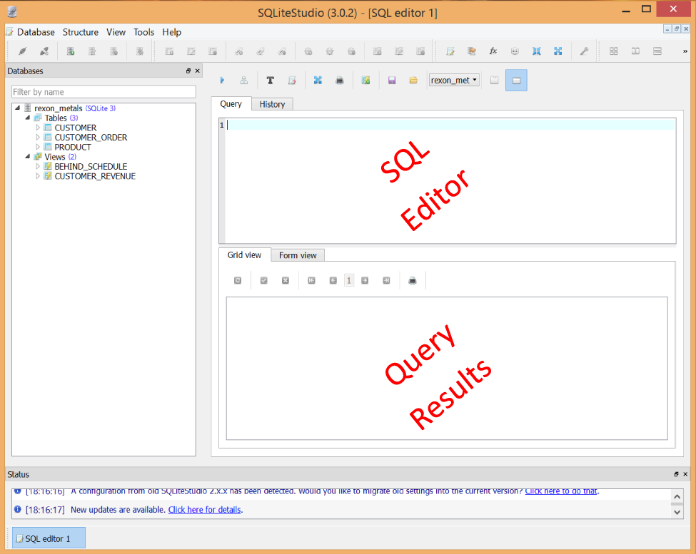
Figure 4-1. The SQL workspace

The SQL Editor pane is where you will write your SQL, and the Query Results pane will display the results of your SQL.

Let’s write our first SQL statement. The most common SQL operation is a SELECT statement, which pulls data from a table and then displays the results. Click on the SQL Editor pane and write the following statement:

SELECT * FROM CUSTOMER;

Click the blue triangle button or hit F9 to execute the SQL.

You just ran your first query, and the results should be displayed in the bottom pane (Figure 4-2).

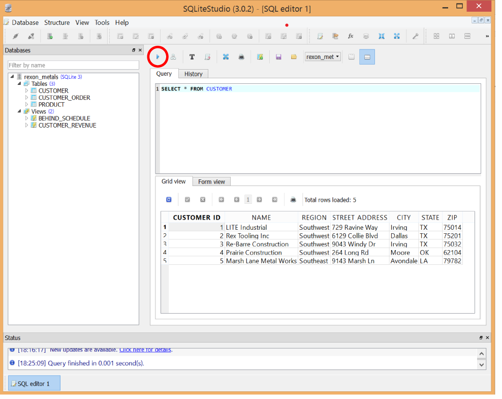
Figure 4-2. Running a SELECT query

Let’s break down exactly what happened. A SELECT statement allows you to choose which columns to pull from a table. So the first part of the SQL shown here should be read as “Select all columns,” where * is a placeholder to specify all columns:

SELECT * FROM CUSTOMER;

And you are getting these columns from the CUSTOMER table:

SELECT * FROM CUSTOMER;

When you execute this SELECT statement, it brings back all the columns from the CUSTOMER table and displays them to you (Figure 4-3).

Figure 4-3. Selecting all records from the CUSTOMER table

You do not have to pull all columns in a SELECT statement. You can also pick and choose only the columns you are interested in. The following query will only pull the CUSTOMER_ID and NAME columns:

SELECT CUSTOMER_ID, NAME FROM CUSTOMER;

And the output will only display those two columns (Figure 4-4).

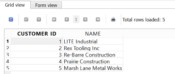
Figure 4-4. Selecting only two columns from a table

Note

A single SQL statement can optionally end with a semicolon (;), as shown in the previous examples. However, the semicolon is necessary to run multiple SQL statements at once, which is helpful when writing data, as covered in Chapter 10.

Being able to pick and choose columns may not seem interesting at the moment, but it allows us to hone in on what we are interested in. Reducing scope to just certain columns will assist with GROUP BY aggregation tasks as well, as we’ll see in Chapter 6.

Expressions in SELECT Statements

The SELECT statement can do far more than simply select columns. You can also do calculations on one or more columns and include them in your query result.

Let’s work with another table called PRODUCT. First, do a SELECT all to see the data (Figure 4-5):

SELECT * FROM PRODUCT;

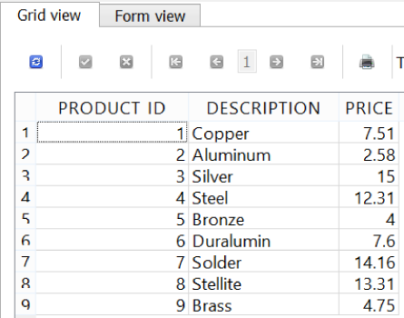
Figure 4-5. The PRODUCT table

Suppose we wanted to generate a calculated column called TAXED_PRICE that is 7% higher than PRICE. We could use a SELECT query to dynamically calculate this for us (Figure 4-6):

SELECT
PRODUCT_ID,
DESCRIPTION,
PRICE,
PRICE * 1.07 AS TAXED_PRICE
FROM PRODUCT;

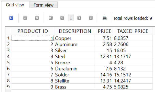
Figure 4-6. Using expressions to calculate a TAXED_PRICE column

Note

Notice in the SELECT statement that we can spread our SQL across multiple lines to make it more legible. The software will ignore extraneous whitespace and separate lines, so we can use them to make our SQL easier to read.

Notice how the TAXED_PRICE column was dynamically calculated in the SELECT query. This column is not stored in the table, but rather calculated and displayed to us every time we run this query. This is a powerful feature of SQL, which allows us to keep the stored data simple and use queries to layer calculations on top of it.

Let’s take a look at our TAXED_PRICE column and break down how it was created. We first see the PRICE is multiplied by 1.07 to calculate the taxed amount. We generate this TAXED_PRICE value for every record:

SELECT
PRODUCT_ID,
DESCRIPTION,
PRICE,
PRICE * 1.07 AS TAXED_PRICE
FROM PRODUCT

Notice too that we gave this calculated value a name using an AS statement (this is known as an alias):

SELECT
PRODUCT_ID,
DESCRIPTION,
PRICE,
PRICE * 1.07 AS TAXED_PRICE
FROM PRODUCT

We can use aliases to give names to expressions. We can also use aliases to apply a new name to an existing column within the query. For example, we can alias the PRICE column to UNTAXED_PRICE (Figure 4-7). This does not actually change the name of the column in the table, but it gives it a new name within the scope of our SELECT statement:

SELECT
PRODUCT_ID,
DESCRIPTION,
PRICE AS UNTAXED_PRICE,
PRICE * 1.07 AS TAXED_PRICE
FROM PRODUCT

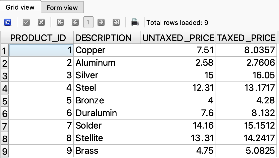
Figure 4-7. Aliasing the PRICE column to UNTAXED_PRICE

Note

When giving names to anything in SQL (whether it is an alias, a column name, a table name, or any other entity), always use an underscore (_) as a placeholder for spaces. It is best practice.

If we were to distribute the results of this SQL statement as a report to our workplace, we would probably want to touch up the rounding on the TAXED_PRICE. Having more than two decimal places may not be desirable. Every database platform has built-in functions to assist with these kinds of operations, and SQLite provides a round() function that accepts two arguments in parentheses separated by a comma: the number to be rounded, and the number of decimal places to round to. To round the TAXED_PRICE to two decimal places, we can pass the multiplication expression PRICE AS UNTAXED_PRICE * 1.07 as the first argument, and a 2 as the second:

SELECT
PRODUCT_ID,
DESCRIPTION,
PRICE AS UNTAXED_PRICE,
round(PRICE AS UNTAXED_PRICE * 1.07, 2) AS TAXED_PRICE
FROM PRODUCT;

Run the statement and you will notice it rounds the TAXED_PRICE, which displays much more nicely with two decimal places (Figure 4-8).

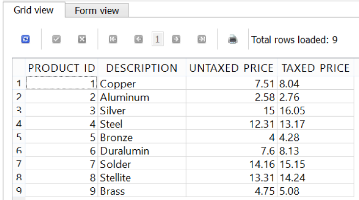
Figure 4-8. Using the round() function to limit decimal places for TAXED_PRICE

Here is a short summary of the mathematical operators you  can use in SQL (we will see these used throughout the book):

Operator	Description	Example
+	Adds two numbers	STOCK + NEW_SHIPMENT
-	Subtracts two numbers	STOCK - DEFECTS
*	Multiplies two numbers	PRICE * 1.07
/	Divides two numbers	STOCK / PALLET_SIZE
%	Divides two numbers, but returns the remainder	STOCK % PALLET_SIZE

Text Concatenation

Expressions do not have to work only with numbers. You can also use expressions with text and other data types. A helpful operator to use with text is concatenation, which merges two or more pieces of data together.    The concatenate operator is specified by a double pipe (||), and you put the data values to concatenate on both sides of it.

For instance, you can concatenate the CITY and STATE fields from the CUSTOMER table as well as put a comma and space between them to create a LOCATION value (Figure 4-9):

SELECT NAME,
CITY || ', ' || STATE AS LOCATION
FROM CUSTOMER;

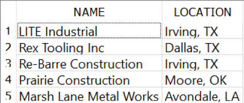
Figure 4-9. Concatenating CITY and STATE

You can even concatenate several fields into a single SHIP_ADDRESS value (Figure 4-10):

SELECT NAME,
STREET_ADDRESS || ' ' || CITY || ', ' || STATE || ' ' || ZIP AS SHIP_ADDRESS
FROM CUSTOMER;

Figure 4-10. Concatenating several fields to create a SHIP_ADDRESS

Concatenation should work with any data type (numbers, dates, etc.) and treat it as text when merging. The ZIP field shown here is a number, but it was implicitly converted to text during concatenation.

More text operations will be covered in the next chapter, but concatenation is definitely an important one.

Note

Many database platforms use double pipes (||) to concatenate, but MySQL and some others require using a CONCAT() function.

Summary

In this chapter, we covered how to use the SELECT statement, the most common SQL operation. It retrieves and transforms data from a table without affecting the table itself. We also learned how to select columns and write expressions. Within expressions, we can use operators and functions to do tasks such as rounding, math, and concatenation.

In the next chapter, we will learn about the WHERE statement, which will allow us to filter records based on criteria we specify.