Hands-On Unsupervised Learning Using Python

Chapter 4. Anomaly Detection

In Chapter 3, we introduced the core dimensionality reduction algorithms and explored their ability to capture the most salient information in the MNIST digits database in significantly fewer dimensions than the original 784 dimensions. Even in just two dimensions, the algorithms meaningfully separated the digits, without using labels. This is the power of unsupervised learning algorithms—they can learn the underlying structure of data and help discover hidden patterns in the absence of labels.

Let’s build an applied machine learning solution using these dimensionality reduction methods. We will turn to the problem we introduced in Chapter 2 and build a credit card fraud detection system without using labels.

In the real world, fraud often goes undiscovered, and only the fraud that is caught provides any labels for the datasets. Moreover, fraud patterns change over time, so supervised systems that are built using fraud labels—like the one we built in Chapter 2—become stale, capturing historical patterns of fraud but failing to adapt to newly emerging patterns.

For these reasons (the lack of sufficient labels and the need to adapt to newly emerging patterns of fraud as quickly as possible), unsupervised learning fraud detection systems are in vogue.

In this chapter, we will build such a solution using some of the dimensionality reduction algorithms we explored in the previous chapter.

Credit Card Fraud Detection

Let’s revisit the credit card transactions problem from Chapter 2.

Prepare the Data

Like we did in Chapter 2, let’s load the credit card transactions dataset, generate the features matrix and labels array, and split the data into training and test sets. We will not use the labels to perform anomaly detection, but we will use the labels to help evaluate the fraud detection systems we build.

As a reminder, we have 284,807 credit card transactions in total, of which 492 are fraudulent, with a positive (fraud) label of one. The rest are normal transactions, with a negative (not fraud) label of zero.

We have 30 features to use for anomaly detection—time, amount, and 28 principal components. And, we will split the dataset into a training set (with 190,820 transactions and 330 cases of fraud) and a test set (with the remaining 93,987 transactions and 162 cases of fraud):

# Load datasets
current_path = os.getcwd()
file = '\\datasets\\credit_card_data\\credit_card.csv'
data = pd.read_csv(current_path + file)

dataX = data.copy().drop(['Class'],axis=1)
dataY = data['Class'].copy()

featuresToScale = dataX.columns
sX = pp.StandardScaler(copy=True)
dataX.loc[:,featuresToScale] = sX.fit_transform(dataX[featuresToScale])

X_train, X_test, y_train, y_test = \
    train_test_split(dataX, dataY, test_size=0.33, \
                    random_state=2018, stratify=dataY)

Define Anomaly Score Function

Next, we need to define a function that calculates how anomalous each transaction is. The more anomalous the transaction is, the more likely it is to be fraudulent, assuming that fraud is rare and looks somewhat different than the majority of transactions, which are normal.

As we discussed in the previous chapter, dimensionality reduction algorithms reduce the dimensionality of data while attempting to minimize the reconstruction error. In other words, these algorithms try to capture the most salient information of the original features in such a way that they can reconstruct the original feature set from the reduced feature set as well as possible. However, these dimensionality reduction algorithms cannot capture all the information of the original features as they move to a lower dimensional space; therefore, there will be some error as these algorithms reconstruct the reduced feature set back to the original number of dimensions.

In the context of our credit card transactions dataset, the algorithms will have the largest reconstruction error on those transactions that are hardest to model—in other words, those that occur the least often and are the most anomalous. Since fraud is rare and presumably different than normal transactions, the fraudulent transactions should exhibit the largest reconstruction error. So let’s define the anomaly score as the reconstruction error. The reconstruction error for each transaction is the sum of the squared differences between the original feature matrix and the reconstructed matrix using the dimensionality reduction algorithm. We will scale the sum of the squared differences by the max-min range of the sum of the squared differences for the entire dataset, so that all the reconstruction errors are within a zero to one range.

The transactions that have the largest sum of squared differences will have an error close to one, while those that have the smallest sum of squared differences will have an error close to zero.

This should be familiar. Like the supervised fraud detection solution we built in Chapter 2, the dimensionality reduction algorithm will effectively assign each transaction an anomaly score between zero and one. Zero is normal and one is anomalous (and most likely to be fraudulent).

Here is the function:

def anomalyScores(originalDF, reducedDF):
    loss = np.sum((np.array(originalDF)-np.array(reducedDF))**2, axis=1)
    loss = pd.Series(data=loss,index=originalDF.index)
    loss = (loss-np.min(loss))/(np.max(loss)-np.min(loss))
    return loss

Define Evaluation Metrics

Although we will not use the fraud labels to build the unsupervised fraud detection solutions, we will use the labels to evaluate the unsupervised solutions we develop. The labels will help us understand just how well these solutions are at catching known patterns of fraud.

As we did in Chapter 2, we will use the precision-recall curve, the average precision, and the auROC as our evaluation metrics.

Here is the function that will plot these results:

def plotResults(trueLabels, anomalyScores, returnPreds = False):
    preds = pd.concat([trueLabels, anomalyScores], axis=1)
    preds.columns = ['trueLabel', 'anomalyScore']
    precision, recall, thresholds = \
        precision_recall_curve(preds['trueLabel'],preds['anomalyScore'])
    average_precision = \
        average_precision_score(preds['trueLabel'],preds['anomalyScore'])

    plt.step(recall, precision, color='k', alpha=0.7, where='post')
    plt.fill_between(recall, precision, step='post', alpha=0.3, color='k')

    plt.xlabel('Recall')
    plt.ylabel('Precision')
    plt.ylim([0.0, 1.05])
    plt.xlim([0.0, 1.0])

    plt.title('Precision-Recall curve: Average Precision = \
    {0:0.2f}'.format(average_precision))

    fpr, tpr, thresholds = roc_curve(preds['trueLabel'], \
                                     preds['anomalyScore'])
    areaUnderROC = auc(fpr, tpr)

    plt.figure()
    plt.plot(fpr, tpr, color='r', lw=2, label='ROC curve')
    plt.plot([0, 1], [0, 1], color='k', lw=2, linestyle='--')
    plt.xlim([0.0, 1.0])
    plt.ylim([0.0, 1.05])
    plt.xlabel('False Positive Rate')
    plt.ylabel('True Positive Rate')
    plt.title('Receiver operating characteristic: \
    Area under the curve = {0:0.2f}'.format(areaUnderROC))
    plt.legend(loc="lower right")
    plt.show()

    if returnPreds==True:
        return preds

Note

The fraud labels and the evaluation metrics will help us assess just how good the unsupervised fraud detection systems are at catching known patterns of fraud—fraud that we have caught in the past and have labels for.

However, we will not be able to assess how good the unsupervised fraud detection systems are at catching unknown patterns of fraud. In other words, there may be fraud in the dataset that is incorrectly labeled as not fraud because the financial company never discovered it.

As you may see already, unsupervised learning systems are much harder to evaluate than supervised learning systems. Often, unsupervised learning systems are judged by their ability to catch known patterns of fraud. This is an incomplete assessment; a better evaluation metric would be to assess them on their ability to identify unknown patterns of fraud, both in the past and in the future.

Since we cannot go back to the financial company and have them evaluate any unknown patterns of fraud we identify, we will have to evaluate these unsupervised systems solely based on how well they detect the known patterns of fraud. It’s important to be mindful of this limitation as we proceed in evaluating the results.

Define Plotting Function

We will reuse the scatterplot function from Chapter 3 to display the separation of points the dimensionality reduction algorithm achieves in just the first two dimensions:

def scatterPlot(xDF, yDF, algoName):
    tempDF = pd.DataFrame(data=xDF.loc[:,0:1], index=xDF.index)
    tempDF = pd.concat((tempDF,yDF), axis=1, join="inner")
    tempDF.columns = ["First Vector", "Second Vector", "Label"]
    sns.lmplot(x="First Vector", y="Second Vector", hue="Label", \
               data=tempDF, fit_reg=False)
    ax = plt.gca()
    ax.set_title("Separation of Observations using "+algoName)

Normal PCA Anomaly Detection

In Chapter 3, we demonstrated how PCA captured the majority of information in the MNIST digits dataset in just a few principal components, far fewer in number than the original dimensions. In fact, with just two dimensions, it was possible to visually separate the images into distinct groups based on the digits they displayed.

Building on this concept, we will now use PCA to learn the underlying structure of the credit card transactions dataset. Once we learn this structure, we will use the learned model to reconstruct the credit card transactions and then calculate how different the reconstructed transactions are from the original transactions. Those transactions that PCA does the poorest job of reconstructing are the most anomalous (and most likely to be fraudulent).

Note

Remember that the features in the credit card transactions dataset we have are already the output of PCA—this is what we were given by the financial company. However, there is nothing unusual about performing PCA for anomaly detection on an already dimensionality-reduced dataset. We just treat the original principal components that we are given as the original features.

Going forward, we will refer to the original principal components that we were given as the original features. Any future mention of principal components will refer to the principal components from the PCA process rather than the original features we were given.

Let’s start by developing a deeper understanding of how PCA—and dimensionality reduction in general—helps perform anomaly detection. As we’ve defined it, anomaly detection relies on reconstruction error. We want the reconstruction error for rare transactions—the ones that are most likely to be fraudulent—to be as high as possible and the reconstruction error for the rest to be as low as possible.

For PCA, the reconstruction error will depend largely on the number of principal components we keep and use to reconstruct the original transactions. The more principal components we keep, the better PCA will be at learning the underlying structure of the original transactions.

However, there is a balance. If we keep too many principal components, PCA may too easily reconstruct the original transactions, so much so that the reconstruction error will be minimal for all of the transactions. If we keep too few principal components, PCA may not be able to reconstruct any of the original transactions well enough—not even the normal, nonfraudulent transactions.

Let’s search for the right number of principal components to keep to build a good fraud detection system.

PCA Components Equal Number of Original Dimensions

First, let’s think about something. If we use PCA to generate the same number of principal components as the number of original features, will we be able to perform anomaly detection?

If you think through this, the answer should be obvious. Recall our PCA example from the previous chapter for the MNIST digits dataset.

When the number of principal components equals the number of original dimensions, PCA captures nearly 100% of the variance/information in the data as it generates the principal components. Therefore, when PCA reconstructs the transactions from the principal components, it will have too little reconstruction error for all the transactions, fraudulent or otherwise. We will not be able to differentiate between rare transactions and normal ones—in other words, anomaly detection will be poor.

To highlight this, let’s apply PCA to generate the same number of principal components as the number of original features (30 for our credit card transactions dataset). This is accomplished with the fit_transform function from Scikit-Learn.

To reconstruct the original transactions from the principal components we generate, we will use the inverse_transform function from Scikit-Learn:

# 30 principal components
from sklearn.decomposition import PCA

n_components = 30
whiten = False
random_state = 2018

pca = PCA(n_components=n_components, whiten=whiten, \
          random_state=random_state)

X_train_PCA = pca.fit_transform(X_train)
X_train_PCA = pd.DataFrame(data=X_train_PCA, index=X_train.index)

X_train_PCA_inverse = pca.inverse_transform(X_train_PCA)
X_train_PCA_inverse = pd.DataFrame(data=X_train_PCA_inverse, \
                                   index=X_train.index)

scatterPlot(X_train_PCA, y_train, "PCA")

Figure 4-1 shows the plot of the separation of transactions using the first two principal components of PCA.

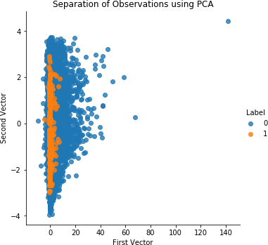
Figure 4-1. Separation of observations using normal PCA and 30 principal components

Let’s calculate the precision-recall curve and the ROC curve:

anomalyScoresPCA = anomalyScores(X_train, X_train_PCA_inverse)
preds = plotResults(y_train, anomalyScoresPCA, True)

With an average precision of 0.11, this is a poor fraud detection solution (see Figure 4-2). It catches very little of the fraud.

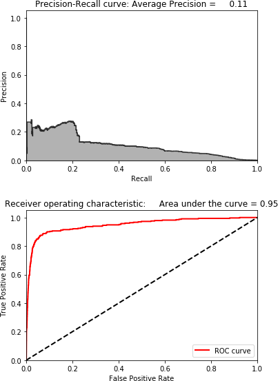
Figure 4-2. Results using 30 principal components

Search for the Optimal Number of Principal Components

Now, let’s perform a few experiments by reducing the number of principal components PCA generates and evaluate the fraud detection results. We need the PCA-based fraud detection solution to have enough error on the rare cases that it can meaningfully separate fraud cases from the normal ones. But the error cannot be so low or so high for all the transactions that the rare and normal transactions are virtually indistinguishable.

After some experimentation, which you can perform using the GitHub code, we find that 27 principal components is the optimal number for this credit card transactions dataset.

Figure 4-3 shows the plot of the separation of transactions using the first two principal components of PCA.

Figure 4-3. Separation of observations using normal PCA and 27 principal components

Figure 4-4 shows the precision-recall curve, average precision, and auROC curve.

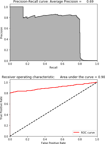
Figure 4-4. Results using normal PCA and 27 principal components

As you can see, we are able to catch 80% of the fraud with 75% precision. This is very impressive considering that we did not use any labels. To make these results more tangible, consider that there are 190,820 transactions in the training set and only 330 are fraudulent.

Using PCA, we calculated the reconstruction error for each of these 190,820 transactions. If we sort these transactions by highest reconstruction error (also referred to as anomaly score) in descending order and extract the top 350 transactions from the list, we can see that 264 of these transactions are fraudulent.

That is a precision of 75%. Moreover, the 264 transactions we caught from the 350 we picked represent 80% of the total fraud in the training set (264 out of 330 fraudulent cases). And, remember that we accomplished this without using labels. This is a truly unsupervised fraud detection solution.

Here is the code to highlight this:

preds.sort_values(by="anomalyScore",ascending=False,inplace=True)
cutoff = 350
predsTop = preds[:cutoff]
print("Precision: ",np.round(predsTop. \
            anomalyScore[predsTop.trueLabel==1].count()/cutoff,2))
print("Recall: ",np.round(predsTop. \
            anomalyScore[predsTop.trueLabel==1].count()/y_train.sum(),2))

The following code summarizes the results:

Precision: 0.75
Recall: 0.8
Fraud Caught out of 330 Cases: 264

Although this is a pretty good solution already, let’s try to develop fraud detection systems using some of the other dimensionality reduction methods.

Sparse PCA Anomaly Detection

Let’s try to use sparse PCA to design a fraud detection solution. Recall that sparse PCA is similar to normal PCA but delivers a less dense version; in other words, sparse PCA provides a sparse representation of the principal components.

We still need to specify the number of principal components we desire, but we must also set the alpha parameter, which controls the degree of sparsity. We will experiment with different values for the principal components and the alpha parameter as we search for the optimal sparse PCA fraud detection solution.

Note that for normal PCA Scikit-Learn used a fit_transform function to generate the principal components and an inverse_transform function to reconstruct the original dimensions from the principal components. Using these two functions, we were able to calculate the reconstruction error between the original feature set and the reconstructed feature set derived from the PCA.

Unfortunately, Scikit-Learn does not provide an inverse_transform function for sparse PCA. Therefore, we must reconstruct the original dimensions after we perform sparse PCA ourselves.

Let’s begin by generating the sparse PCA matrix with 27 principal components and the default alpha parameter of 0.0001:

# Sparse PCA
from sklearn.decomposition import SparsePCA

n_components = 27
alpha = 0.0001
random_state = 2018
n_jobs = -1

sparsePCA = SparsePCA(n_components=n_components, \
                alpha=alpha, random_state=random_state, n_jobs=n_jobs)

sparsePCA.fit(X_train.loc[:,:])
X_train_sparsePCA = sparsePCA.transform(X_train)
X_train_sparsePCA = pd.DataFrame(data=X_train_sparsePCA, index=X_train.index)

scatterPlot(X_train_sparsePCA, y_train, "Sparse PCA")

Figure 4-5 shows the scatterplot for sparse PCA.

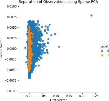
Figure 4-5. Separation of observations using sparse PCA and 27 principal components

Now let’s generate the original dimensions from the sparse PCA matrix by simple matrix multiplication of the sparse PCA matrix (with 190,820 samples and 27 dimensions) and the sparse PCA components (a 27 x 30 matrix), provided by Scikit-Learn library. This creates a matrix that is the original size (a 190,820 x 30 matrix). We also need to add the mean of each original feature to this new matrix, but then we are done.

From this newly derived inverse matrix, we can calculate the reconstruction errors (anomaly scores) as we did with normal PCA:

X_train_sparsePCA_inverse = np.array(X_train_sparsePCA). \
    dot(sparsePCA.components_) + np.array(X_train.mean(axis=0))
X_train_sparsePCA_inverse = \
    pd.DataFrame(data=X_train_sparsePCA_inverse, index=X_train.index)

anomalyScoresSparsePCA = anomalyScores(X_train, X_train_sparsePCA_inverse)
preds = plotResults(y_train, anomalyScoresSparsePCA, True)

Now, let’s generate the precision-recall curve and ROC curve.

Figure 4-6. Results using sparse PCA and 27 principal components

As Figure 4-6 shows, the results are identical to those of normal PCA. This is expected since normal and sparse PCA are very similar—the latter is just a sparse representation of the former.

Using the GitHub code, you can experiment by changing the number of principal components generated and the alpha parameter, but, based on our experimentation, this is the best sparse PCA-based fraud detection solution.

Kernel PCA Anomaly Detection

Now let’s design a fraud detection solution using kernel PCA, which is a nonlinear form of PCA and is useful if the fraud transactions are not linearly separable from the nonfraud transactions.

We need to specify the number of components we would like to generate, the kernel (we will use the RBF kernel as we did in the previous chapter), and the gamma (which is set to 1/n_features by default, so 1/30 in our case). We also need to set the fit_inverse_transform to true to apply the built-in inverse_transform function provided by Scikit-Learn.

Finally, because kernel PCA is so expensive to train with, we will train on just the first two thousand samples in the transactions dataset. This is not ideal but it is necessary to perform experiments quickly.

We will use this training to transform the entire training set and generate the principal components. Then, we will use the inverse_transform function to recreate the original dimension from the principal components derived by kernel PCA:

# Kernel PCA
from sklearn.decomposition import KernelPCA

n_components = 27
kernel = 'rbf'
gamma = None
fit_inverse_transform = True
random_state = 2018
n_jobs = 1

kernelPCA = KernelPCA(n_components=n_components, kernel=kernel, \
                gamma=gamma, fit_inverse_transform= \
                fit_inverse_transform, n_jobs=n_jobs, \
                random_state=random_state)

kernelPCA.fit(X_train.iloc[:2000])
X_train_kernelPCA = kernelPCA.transform(X_train)
X_train_kernelPCA = pd.DataFrame(data=X_train_kernelPCA, \
                                 index=X_train.index)

X_train_kernelPCA_inverse = kernelPCA.inverse_transform(X_train_kernelPCA)
X_train_kernelPCA_inverse = pd.DataFrame(data=X_train_kernelPCA_inverse, \
                                         index=X_train.index)

scatterPlot(X_train_kernelPCA, y_train, "Kernel PCA")

Figure 4-7 shows the scatterplot for kernel PCA.

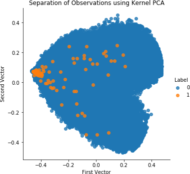
Figure 4-7. Separation of observations using kernel PCA and 27 principal components

Now, let’s calculate the anomaly scores and print the results.

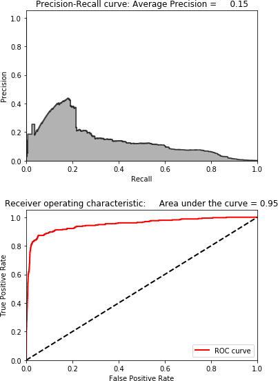
Figure 4-8. Results using kernel PCA and 27 principal components

As Figure 4-8 shows, the results are far worse than those for normal PCA and sparse PCA. While it was worth experimenting with kernel PCA, we will not use this solution for fraud detection given that we have better performing solutions from earlier.

Note

We will not build an anomaly detection solution using SVD because the solution is very similar to that of normal PCA. This is expected—PCA and SVD are closely related.

Instead, let’s move to random projection-based anomaly detection.

Gaussian Random Projection Anomaly Detection

Now, let’s try to develop a fraud detection solution using Gaussian random projection. Remember that we can set either the number of components we want or the eps parameter, which controls the quality of the embedding derived based on the Johnson–Lindenstrauss lemma.

We will choose to explicitly set the number of components. Gaussian random projection trains very quickly, so we can train on the entire training set.

As with sparse PCA, we will need to derive our own inverse_transform function because none is provided by Scikit-Learn:

# Gaussian Random Projection
from sklearn.random_projection import GaussianRandomProjection

n_components = 27
eps = None
random_state = 2018

GRP = GaussianRandomProjection(n_components=n_components, \
                               eps=eps, random_state=random_state)

X_train_GRP = GRP.fit_transform(X_train)
X_train_GRP = pd.DataFrame(data=X_train_GRP, index=X_train.index)

scatterPlot(X_train_GRP, y_train, "Gaussian Random Projection")

Figure 4-9 shows the scatterplot for Gaussian random projection. Figure 4-10 displays the results for Gaussian random projection.

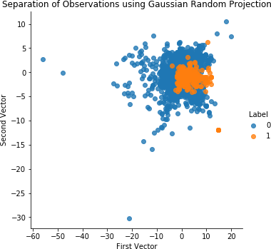
Figure 4-9. Separation of observations using Gaussian random projection and 27 components

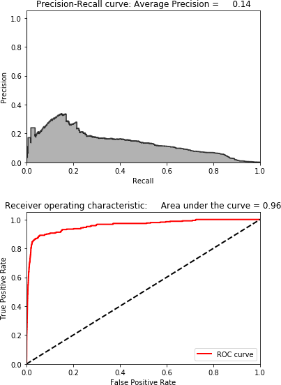
Figure 4-10. Results using Gaussian random projection and 27 components

These results are poor, so we won’t use Gaussian random projection for fraud detection.

Sparse Random Projection Anomaly Detection

Let’s try to design a fraud detection solution using sparse random projection.

We will designate the number of components we want (instead of setting the eps parameter). And, like with Gaussian random projection, we will use our own inverse_transform function to create the original dimensions from the sparse random projection-derived components:

# Sparse Random Projection

from sklearn.random_projection import SparseRandomProjection

n_components = 27
density = 'auto'
eps = .01
dense_output = True
random_state = 2018

SRP = SparseRandomProjection(n_components=n_components, \
        density=density, eps=eps, dense_output=dense_output, \
                                random_state=random_state)

X_train_SRP = SRP.fit_transform(X_train)
X_train_SRP = pd.DataFrame(data=X_train_SRP, index=X_train.index)

scatterPlot(X_train_SRP, y_train, "Sparse Random Projection")

Figure 4-11 shows the scatterplot for sparse random projection. Figure 4-12 displays the results for sparse random projection.

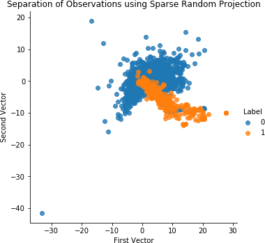
Figure 4-11. Separation of observations using sparse random projection and 27 components

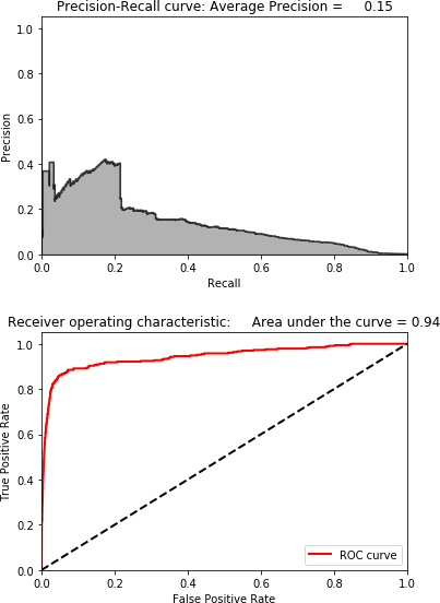
Figure 4-12. Results using sparse random projection and 27 components

As with Gaussian random projection, these results are poor. Let’s continue to build anomaly detection systems using other dimensionality reduction methods.

Nonlinear Anomaly Detection

So far, we have developed fraud detection solutions using linear dimensionality reduction methods such as normal PCA, sparse PCA, Gaussian random projection, and sparse random projection. We also developed a solution using the nonlinear version of PCA—kernel PCA.

At this point, PCA is by far the best solution.

We could turn to nonlinear dimensionality reduction algorithms, but the open source versions of these algorithms run very slowly and are not viable for fast fraud detection. Therefore, we will skip this and go directly to nondistance-based dimensionality reduction methods: dictionary learning and independent component analysis.

Dictionary Learning Anomaly Detection

Let’s use dictionary learning to develop a fraud detection solution. Recall that, in dictionary learning, the algorithm learns the sparse representation of the original data. Using the vectors in the learned dictionary, each instance in the original data can be reconstructed as a weighted sum of these learned vectors.

For anomaly detection, we want to learn an undercomplete dictionary so that the vectors in the dictionary are fewer in number than the original dimensions. With this constraint, it will be easier to reconstruct the more frequently occurring normal transactions and much more difficult to construct the rarer fraud transactions.

In our case, we will generate 28 vectors (or components). To learn the dictionary, we will feed in 10 batches, where each batch has 200 samples.

We will need to use our own inverse_transform function, too:

# Mini-batch dictionary learning
from sklearn.decomposition import MiniBatchDictionaryLearning

n_components = 28
alpha = 1
batch_size = 200
n_iter = 10
random_state = 2018

miniBatchDictLearning = MiniBatchDictionaryLearning( \
    n_components=n_components, alpha=alpha, batch_size=batch_size, \
    n_iter=n_iter, random_state=random_state)

miniBatchDictLearning.fit(X_train)
X_train_miniBatchDictLearning = \
    miniBatchDictLearning.fit_transform(X_train)
X_train_miniBatchDictLearning = \
    pd.DataFrame(data=X_train_miniBatchDictLearning, index=X_train.index)

scatterPlot(X_train_miniBatchDictLearning, y_train, \
            "Mini-batch Dictionary Learning")

Figure 4-13 shows the scatterplot for dictionary learning. Figure 4-14 shows the results for dictionary learning.

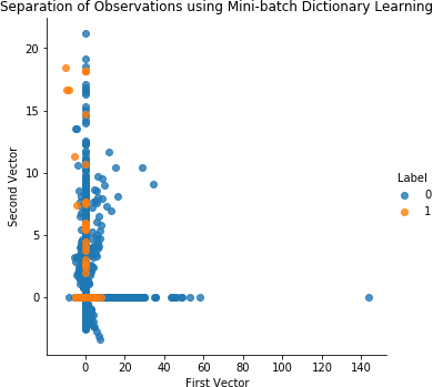
Figure 4-13. Separation of observations using dictionary learning and 28 components

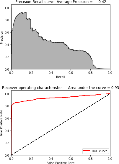
Figure 4-14. Results using dictionary learning and 28 components

These results are much better than those for kernal PCA, Gaussian random projection, and sparse random projection but are no match for those of normal PCA.

You can experiment with the code on GitHub to see if you could improve on this solution, but, for now, PCA remains the best fraud detection solution for this credit card transactions dataset.

ICA Anomaly Detection

Let’s use ICA to design our last fraud detection solution.

We need to specify the number of components, which we will set to 27. Scikit-Learn provides an inverse_transform function so we do not need to use our own:

# Independent Component Analysis

from sklearn.decomposition import FastICA

n_components = 27
algorithm = 'parallel'
whiten = True
max_iter = 200
random_state = 2018

fastICA = FastICA(n_components=n_components, \
    algorithm=algorithm, whiten=whiten, max_iter=max_iter, \
    random_state=random_state)

X_train_fastICA = fastICA.fit_transform(X_train)
X_train_fastICA = pd.DataFrame(data=X_train_fastICA, index=X_train.index)

X_train_fastICA_inverse = fastICA.inverse_transform(X_train_fastICA)
X_train_fastICA_inverse = pd.DataFrame(data=X_train_fastICA_inverse, \
                                       index=X_train.index)

scatterPlot(X_train_fastICA, y_train, "Independent Component Analysis")

Figure 4-15 shows the scatterplot for ICA. Figure 4-16 shows the results for ICA.

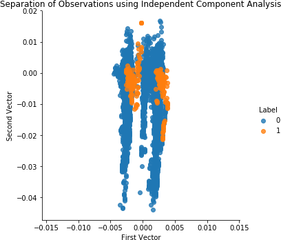
Figure 4-15. Separation of observations using ICA and 27 components

Figure 4-16. Results using ICA and 27 components

These results are identical to those of normal PCA. The fraud detection solution using ICA matches the best solution we’ve developed so far.

Fraud Detection on the Test Set

Now, to evaluate our fraud detection solutions, let’s apply them to the never-before-seen test set. We will do this for the top three solutions we’ve developed: normal PCA, ICA, and dictionary learning. We will not use sparse PCA because it is very similar to the normal PCA solution.

Normal PCA Anomaly Detection on the Test Set

Let’s start with normal PCA. We will use the PCA embedding that the PCA algorithm learned from the training set and use this to transform the test set. We will then use the Scikit-Learn inverse_transform function to recreate the original dimensions from the principal components matrix of the test set.

By comparing the original test set matrix with the newly reconstructed one, we can calculate the anomaly scores (as we’ve done many times before in this chapter):

# PCA on Test Set
X_test_PCA = pca.transform(X_test)
X_test_PCA = pd.DataFrame(data=X_test_PCA, index=X_test.index)

X_test_PCA_inverse = pca.inverse_transform(X_test_PCA)
X_test_PCA_inverse = pd.DataFrame(data=X_test_PCA_inverse, \
                                  index=X_test.index)

scatterPlot(X_test_PCA, y_test, "PCA")

Figure 4-17 shows the scatterplot for PCA on the test set. Figure 4-18 displays the results for PCA on the test set.

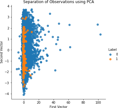
Figure 4-17. Separation of observations using PCA and 27 components on the test set

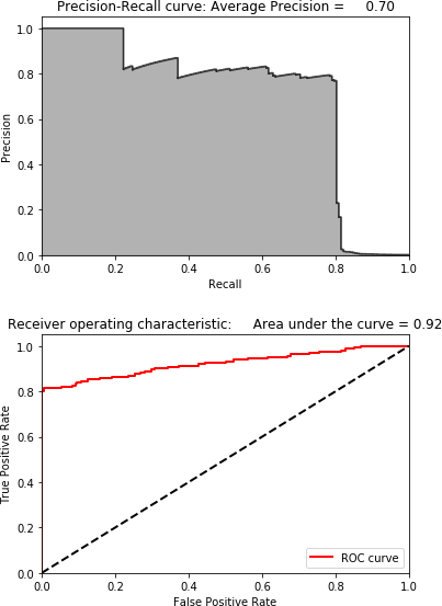
Figure 4-18. Results using PCA and 27 components on the test set

These are impressive results. We are able to catch 80% of the known fraud in the test set with an 80% precision—all without using any labels.

ICA Anomaly Detection on the Test Set

Let’s now move to ICA and perform fraud detection on the test set:

# Independent Component Analysis on Test Set
X_test_fastICA = fastICA.transform(X_test)
X_test_fastICA = pd.DataFrame(data=X_test_fastICA, index=X_test.index)

X_test_fastICA_inverse = fastICA.inverse_transform(X_test_fastICA)
X_test_fastICA_inverse = pd.DataFrame(data=X_test_fastICA_inverse, \
                                      index=X_test.index)

scatterPlot(X_test_fastICA, y_test, "Independent Component Analysis")

Figure 4-19 shows the scatterplot for ICA on the test set. Figure 4-20 shows the results for ICA on the test set.

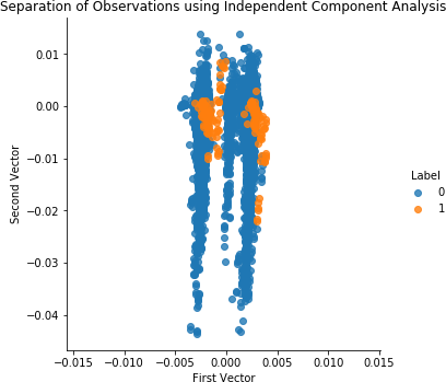
Figure 4-19. Separation of observations using ICA and 27 components on the test set

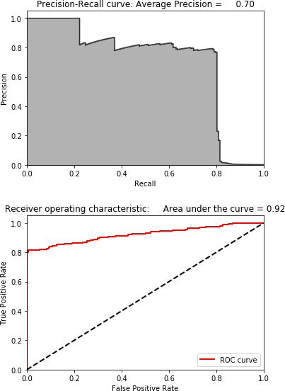
Figure 4-20. Results using ICA and 27 components on the test set

The results are identical to normal PCA and thus quite impressive.

Dictionary Learning Anomaly Detection on the Test Set

Let’s now turn to dictionary learning, which did not perform as well as normal PCA and ICA but is worth a final look:

X_test_miniBatchDictLearning = miniBatchDictLearning.transform(X_test)
X_test_miniBatchDictLearning = \
    pd.DataFrame(data=X_test_miniBatchDictLearning, index=X_test.index)

scatterPlot(X_test_miniBatchDictLearning, y_test, \
            "Mini-batch Dictionary Learning")

Figure 4-21 shows the scatterplot for dictionary learning on the test set. Figure 4-22 displays the results for dictionary learning on the test set.

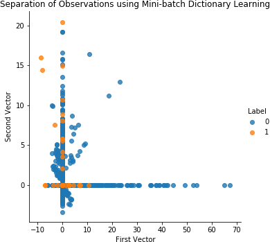
Figure 4-21. Separation of observations using dictionary learning and 28 components on the test set

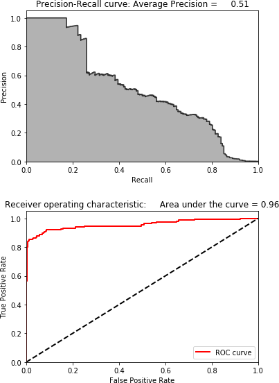
Figure 4-22. Results using dictionary learning and 28 components on the test set

While the results are not terrible—we can catch 80% of the fraud with a 20% precision—they fall far short of the results from normal PCA and ICA.

Conclusion

In this chapter, we used the core dimensionality reduction algorithms from the previous chapter to develop fraud detection solutions for the credit card transactions dataset from Chapter 2.

In Chapter 2 we used labels to build a fraud detection solution, but we did not use any labels during the training process in this chapter. In other words, we built an applied fraud detection system using unsupervised learning.

While not all the dimensionality reduction algorithms performed well on this credit card transactions dataset, two performed remarkably well—normal PCA and ICA.

Normal PCA and ICA caught over 80% of the known fraud with an 80% precision. By comparison, the best-performing supervised learning-based fraud detection system from Chapter 2 caught nearly 90% of the known fraud with an 80% precision. The unsupervised fraud detection system is only marginally worse than the supervised system at catching known patterns of fraud.

Recall that unsupervised fraud detection systems require no labels for training, adapt well to changing fraud patterns, and can catch fraud that had gone previously undiscovered. Given these additional advantages, the unsupervised learning-based solution will generally perform better than the supervised learning-based solution at catching known and unknown or newly emerging patterns of fraud in the future, although using both in tandem is best.

Now that we’ve covered dimensionality reduction and anomaly detection, let’s explore clustering, another major concept in the field of unsupervised learning.