Intermediate Financial Theory, 3rd Edition

The x_t random variable thus moves slowly (depending on ϕ), with a tendency to return to its mean value. Lastly, mean reversion is captured by assuming cov(η_t+1, u_t+1)=σ_ηu<0, which translates, as per below, into a statement about risky return autocorrelations:

$\begin{array}{l}0>{\sigma }_{\eta u}=\mathrm{cov}({\tilde{u}}_{t+1},{\tilde{\eta }}_{t+1})={\mathrm{cov}}_t[({\tilde{r}}_{t+1}-E_t{\tilde{r}}_{t+1}),({\tilde{x}}_{t+1}-\overline{x}-\varphi (x_t-\overline{x}))]\hfill \\ ={\mathrm{cov}}_t({\tilde{r}}_{t+1},{\tilde{x}}_{t+1})\hfill \\ ={\mathrm{cov}}_t\left({\tilde{r}}_{t+1},E_t{\tilde{r}}_{t+2}-r_f+\frac{{\sigma }_u^2}{2}\right)\hfill \\ ={\mathrm{cov}}_t\left({\tilde{r}}_{t+1},{\tilde{r}}_{t+2}-{\tilde{u}}_{t+2}-r_f+\frac{{\sigma }_u^2}{2}\right)\hfill \\ ={\mathrm{cov}}_t({\tilde{r}}_{t+1},{\tilde{r}}_{t+2})\hfill \end{array}$

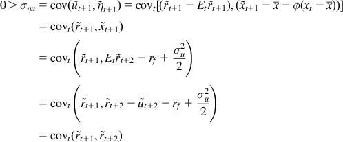
a high return today reduces expected returns next period. Thus,

${\mathrm{var}}_t({\tilde{r}}_{t+1}+{\tilde{r}}_{t+2})=2{\mathrm{var}}_t({\tilde{r}}_{t+1})+2{\mathrm{cov}}_t({\tilde{r}}_{t+1},{\tilde{r}}_{t+2})<2{\mathrm{var}}_t(r_{t+1})$

in contrast to the independence case. More generally, for all horizons k,

$\frac{{\mathrm{var}}_t({\tilde{r}}_{t+1}+{\tilde{r}}_{t+2}+\cdots +{\tilde{r}}_t}{}$