Let's start out with a plot of the time series using base R:
> plot(climate_ts, main = "CO2 and Temperature Deviation")
The output of the preceding command is as follows:
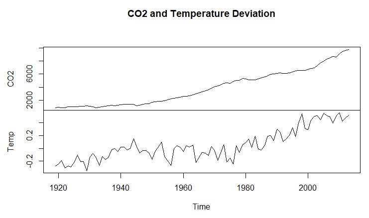
It appears that CO2 levels really started to increase after World War II and there's a rapid rise in temperature anomalies in the mid-1970s. There doesn't appear to be any obvious outliers, and variation over time appears constant. Using the standard procedure, we can see that the two series are highly correlated, as follows:
> cor(climate_temp) CO2 Temp CO2 1.0000000 0.8404215 Temp 0.8404215 1.0000000
As discussed earlier, this is nothing to jump for joy ...

