Multivariate Time Series Analysis and Applications

2Vector time series models

Although as shown in Chapter 1, a stationary vector time series process Z_t that is purely nondeterministic can always be written as a moving average representation, and an invertible vector time series process can always be written as an autoregressive representation; they involve an infinite number of coefficient matrices in the representation. In practice, with a finite number of observations, we will construct a time series model with a finite number of coefficient matrices. Specifically, we will present VMA(q), VAR(p), VARMA(p, q), and VARMA(p, q) × (P, Q)_s models in this chapter. After introducing the properties of these models, we will discuss their parameter estimation and forecasting. We will also introduce the concept of multivariate time series (MTS) outliers and their detections. Detailed empirical examples will be given.

2.1 Vector moving average processes

The m‐dimensional vector moving average process or model in the order of q, shortened to VMA(q), is given by

(2.1)

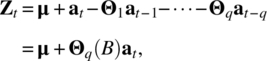
where Θ_q(B) = I − Θ₁B − ⋯ − Θ_qB^q, a_t is a sequence of the m‐dimensional vector white noise process, VWN(0, Σ), with mean vector, 0, and covariance matrix function

(2.2)

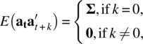
and Σ is a m × m symmetric positive‐definite matrix. The VMA(q) model is clearly stationary with the mean ...