Chapter 4. Cloud
Few technology trends have had the impact that cloud computing has had on the IT industry—save perhaps virtualization, which is a foundational technology for cloud computing. As a network engineer, you may be asking yourself, “What does cloud computing have to do with me?” Some network engineers may dismiss cloud computing, feeling like their skills aren’t needed for cloud-based environments. Others, including the authors, feel quite differently.
Networking is every bit as important “in the cloud” as it is for an on-premises environment. In fact, some might say that networking is even more important in the cloud. Additionally, to truly reap the benefits of cloud computing—easy scale-in/scale-out, on-demand resources, and ephemeral environments, among others—you really need to embrace automation. It’s only natural, then, that a book on network automation and programmability discusses the role of cloud computing in the context of network automation.
Entire tomes have been written and will probably continue to be written about the various cloud providers, the services these cloud providers offer, how to architect solutions for the cloud providers, and more. With that in mind, this chapter aims to be a bit more compact and provide only the key essentials you need as a network engineer to add cloud computing to your arsenal of tools for solving the problems you encounter on a daily basis.
The best place to start is by establishing a baseline definition of cloud computing.
Brief Definition of Cloud Computing
While many definitions of cloud computing exist (one need only perform a web search for “what is cloud computing”), one of the quintessential definitions comes from the United States Department of Commerce—specifically, from the National Institute of Standards and Technology (NIST). NIST’s definition of cloud computing, as contained in Special Publication 800-145, is a multifaceted definition that tackles key characteristics of cloud computing as well as service and deployment models. The NIST definition describes all these things in a vendor-agnostic manner.
NIST defines five essential characteristics of cloud computing:
- On-demand self-service
-
Users (NIST refers to “consumers”) should be able to provision their own resources from the cloud provider as needed, without needing to involve human interaction (in other words, without having to file a service ticket!).
- Broad network access
-
Cloud environments are inherently networked environments, accessible over the network. This is where the statement that networking is just as important in the cloud originates—without ubiquitous network access, it’s not cloud computing.
- Resource pooling
-
Cloud provider resources are pooled and served to multiple tenants automatically. This includes physical and virtual resources and applies not only to computing capacity but also to storage and networking.
- Rapid elasticity
-
Cloud resources should be able to scale “infinitely” (from the user’s perspective, they appear to be unlimited). Scaling up or scaling down, based on demand, should be possible—even automatic, in some cases.
- Measured service
-
Cloud resources are metered, and users are charged for what they use. Usage can be monitored, controlled, and reported.
The NIST definition also defines three service models:
- Software as a service (SaaS)
-
The “service” supplied here is access to a provider’s applications, likely running on a cloud infrastructure. However, the cloud infrastructure is not exposed to the users; only the application and application interface(s) are exposed to the users. Examples of SaaS offerings include Salesforce, Okta, and Microsoft 365.
- Platform as a service (PaaS)
-
In the case of PaaS, users have access to a platform—comprising “programming languages, libraries, services, and tools supported by the provider” (to use NIST’s wording)—onto which they can deploy applications. These applications may be acquired by the user (purchased or licensed) or created by the user. The users do not have access to the cloud infrastructure under this platform; only the platform’s interface(s) are exposed to the users. Examples of PaaS offerings are Heroku and AWS Elastic Beanstalk.
- Infrastructure as a service (IaaS)
-
The last service model is IaaS, in which users have access to provision compute, storage, networking, security, and other fundamental resources in order to deploy arbitrary software, up to and including OS instances and applications. The users do not have access to the cloud infrastructure directly, but have access to control the way fundamental resources are provisioned. For example, users don’t have access to the underlying components that make an Amazon Virtual Private Cloud (VPC) work, but users do have the ability to create and configure VPCs. Real-world examples of IaaS offerings include many aspects of AWS, many services provided by Microsoft Azure, and multiple services offered by Google Cloud.
Note
The wording we use in our examples of IaaS—“many aspects of” or “many services provided by”—is intentional. All, or nearly all, cloud providers offer a variety of services that fall into different service models. Some offerings are squarely IaaS, while others may be classified as PaaS or even SaaS.
Finally, the NIST definition discusses deployment models:
- Private cloud
-
For a private cloud, the cloud infrastructure—defined by NIST as the collection of hardware and software that enables the five essential characteristics of cloud computing—is provisioned for use by a single entity, like a corporation. This infrastructure may be on premises or off premises; the location doesn’t matter. Similarly, it may be operated by the organization or someone else. The key distinction here is the intended audience, which is only the organization or entity.
- Community cloud
-
A community cloud is provisioned for use by a shared community of users—a group of companies with shared regulatory requirements, perhaps, or organizations that share a common cause. It may be owned by one or more of the organizations in the community or a third party. Likewise, it may be operated by one or more members of the community or by a third party and does not distinguish between on premises and off premises.
- Public cloud
-
The cloud infrastructure of a public cloud is provisioned for use by the general public. Ownership, management, and operation of the public cloud may be by a business, a government organization, an academic entity, or a combination of these. A public cloud exists on the premises of the provider (the organization that owns, manages, and operates the cloud infrastructure).
- Hybrid cloud
-
A hybrid cloud is simply a composition of two or more distinct cloud infrastructures that are joined in some fashion, either by standardized or proprietary technology that enables some level of data and application portability among the cloud infrastructures.
As you can see from these three aspects—the essential characteristics of cloud computing, the service models by which it is offered to users, and the deployment models by which it is provisioned for an audience—cloud computing is multifaceted.
In this chapter, we focus primarily on public cloud deployment models that typically fall within the IaaS service model.
Note
We say “typically fall within the IaaS service model” because some service offerings can’t be cleanly categorized as IaaS or PaaS. The industry has even coined new terms, like functions as a service (FaaS) or database as a service (DBaaS), to describe offerings that don’t cleanly fall into one of the categories defined by NIST.
It’s now appropriate, having defined the various forms of cloud computing, to shift your attention to the fundamentals of networking in the cloud.
Networking Fundamentals in the Cloud
Although networking operates a bit differently in cloud environments, in the end, cloud networking is just networking. Many (most?) of the skills you’ve developed as a network engineer continue to apply when dealing with networking in cloud environments, and the hard-won knowledge and experience you’ve gathered won’t go to waste.
In particular, you’ll no longer need to worry much about low-level details (i.e., you don’t need to know how the network constructs, such as virtual networks, are implemented—just use the abstractions), but things like routing protocols, routing topologies, network topology design, and IP address planning remain very much needed. Let’s start with a look at some of the key building blocks for cloud networking.
Cloud Networking Building Blocks
Although the specific details vary among cloud providers, all the major ones offer some basic (generic) features and functionalities:
- Logical network isolation
-
Much in the same way that encapsulation protocols like VXLAN, Generic Routing Encapsulation (GRE), and others create overlay networks that isolate logical network traffic from the physical network, all the major cloud providers offer network isolation mechanisms. On AWS, this is a Virtual Private Cloud (VPC), which we better explain in “A small cloud network topology”; on Azure, it’s a Virtual Network (also known as a VNet); and on Google Cloud, it’s just called a Network. Regardless of the name, the basic purpose is the same: to provide a means whereby logical networks can be isolated and segregated from one another. These logical networks provide complete segregation from all other logical networks, but—as you’ll see in a moment—can still be connected in various ways to achieve the desired results.
- Public and private addressing
-
Workloads can be assigned public (routable) addresses or private (nonroutable) addresses. See RFC 1918 and RFC 6598. The cloud provider supplies mechanisms for providing internet connectivity to both public and private workloads. All of this is typically done at the logical network layer, meaning that each logical network can have its own IP address assignments. Overlapping IP address spaces are permitted among multiple logical networks.
- Persistent addressing
-
Network addresses can be allocated to a cloud provider customer’s account, and then assigned to a workload. Later, that same address can be unassigned from the workload and assigned to a different workload, but the address remains constant and persistent until it is released from the customer’s account back to the cloud provider. Elastic IP addresses (EIPs) on AWS or public IP addresses on Azure are examples.
- Complex topologies
-
The logical network isolation building blocks (VPCs on AWS, VNets on Azure, Networks on Google Cloud) can be combined in complex ways, and network engineers have control over how traffic is routed among these building blocks. Large companies with significant cloud resources in use may end up with multiple hundreds of logical networks, along with site-to-site VPN connections and connections back to on-premises (self-managed) networks. The level of complexity here can easily rival or surpass even the most comprehensive on-premises networks, and the need for skilled network engineers who know how to design these networks and automate their implementation is great.
- Load balancing
-
Cloud providers offer load-balancing solutions that are provisioned on demand and provide Layer 4 (TCP/UDP) load balancing, Layer 7 (HTTP) load balancing (with or without TLS termination), internal load balancing (internal to a customer’s private/nonroutable address space within a VPC or VNet), or external load balancing (for traffic originating from internet-based sources).
Note
For network engineers who are just getting accustomed to cloud networking, Timothy McConnaughy’s The Hybrid Cloud Handbook for AWS (Carpe DMVPN) is a good introduction to the basics of AWS networking.
Numerous other network services are available from the major cloud providers that aren’t discussed here—including API gateways, network-level access controls, instance-level access controls, and even support for third-party network appliances to perform additional functions. Further, all of these network services are available on demand. Users need only log into their cloud management console, use the cloud provider’s CLI tool, interact with the cloud provider’s APIs, or even use one of any number of cloud automation tools to instantiate one or more of these network services (we discuss these tools in more detail in Chapter 12). Our goal in this chapter isn’t to try to explain all of them but rather to help you see how these pieces fit into the overall picture of network programmability and automation.
With this high-level understanding of the cloud networking building blocks in place, let’s shift our attention to a few examples of how you would go about assembling these building blocks.
Cloud Network Topologies
To help solidify the concepts behind the relatively generic constructs described in the previous section, this section narrows the discussion to the actual offerings from one specific public cloud provider: AWS. AWS is the largest of the public cloud providers, both in terms of the breadth of services offered as well as in terms of market adoption (according to a June 2022 Gartner report, AWS had 38.9% of the total cloud market). Therefore, it’s a good place to start. However, similar concepts apply to other cloud providers, including Microsoft Azure, Google Cloud Platform, Alibaba Cloud, Oracle Cloud, DigitalOcean, and others.
Tip
Plenty of great resources online can help you learn about cloud providers’ best design practices. For AWS, you can get started with the AWS Well-Architected framework.
This section discusses four scenarios:
-
A small environment involving only a single logical network
-
A medium-sized environment involving a few to several logical networks
-
A larger environment dealing with multiple dozens of logical networks
-
A hybrid environment involving both on-premises and cloud-based networks
A small cloud network topology
Our small cloud network topology leverages only a single VPC. At first, this might seem limiting—will a single VPC be able to scale enough? Is this sort of topology valid for only the very smallest of customers, those who have only a few workloads in the public cloud?
Note
The virtual network construct, like AWS VPC, is the key building block for cloud networking. Even though each cloud provider implements this construct a bit differently, the basic idea is the same: a virtual network is a logical network (with some Layer 2 and 3 features) that can be used to isolate workloads from one another. All the cloud services are attached to a virtual network so they can communicate with one another (assuming the appropriate network access controls are in place).
In thinking about scalability, consider these dimensions:
- IP addressing
-
When you create a VPC, you must specify a Classless Inter-Domain Routing (CIDR) block. It’s recommended to use blocks from the ranges specified in RFC 1918 and RFC 6598. The block can range in size from a /16 (supplying up to 65,536 IP addresses) all the way to a /28 (supplying only 16 IP addresses). Further, you can add CIDR blocks—up to four additional, nonoverlapping blocks for a total of five CIDR blocks in a VPC—to provide even more available IP addresses. Five /16 CIDR blocks would provide over 300,000 IP addresses.
- Bandwidth
-
AWS supplies two mechanisms for connecting workloads to the internet. For workloads on a public subnet, you use an internet gateway. AWS describes this component as “a horizontally scaled, redundant, and highly available VPC component” that “does not cause availability risks or bandwidth constraints”; see the Amazon VPC documentation. For workloads on a private subnet, you typically use a NAT gateway, which according to AWS scales up to 100 Gbps. NAT stands for network address translation, which is the name given to the process of mapping private (nonroutable) IP addresses to public (routable) IP addresses.
Note
For the purposes of this book, a public subnet is defined as a subnet that is connected to or has a default route to an internet gateway. Typically, a public subnet is also configured to assign a routable IP address to resources. A private subnet is defined as a subnet that is connected to or has a default route to a NAT gateway (or a self-managed NAT instance). A private subnet is also typically configured to use only nonroutable (RFC 1918/6598) IP addresses.
- Availability
-
A single VPC can span multiple availability zones but cannot span multiple regions. A region in AWS parlance is a grouping of data centers. An availability zone (AZ) within a region is a physically separate, isolated logical cluster of data centers. Each availability zone has independent power, cooling, and redundant network connectivity. AZs within a region have high-speed, low-latency connections among them. The idea behind spanning multiple AZs is that a failure in one AZ of a region will generally not affect other AZs in a region, thus giving you the ability to withstand failures in a more resilient way. A subnet is limited to a single AZ and cannot span AZs.
- Security
-
AWS offers network-level traffic-filtering mechanisms (called network access control lists) and host-level traffic-filtering mechanisms (called security groups). Network access control lists (network ACLs, or NACLs) are stateless and operate at the network level (specifically, the subnet level). NACL rules are processed in order, according to the rule’s assigned number (think of the number as a priority: the lowest-numbered rule decides first or has the highest priority). Security groups, on the other hand, are stateful, operate at the instance level, and evaluate all the rules before deciding whether to allow traffic. NACLs and security groups can—and should be—used together to help provide the strongest level of control over the types of traffic that are or are not allowed between workloads within a VPC.
None of these areas presents any significant limitation or constraint, proving that even a cloud network design leveraging a single VPC can scale to thousands of workloads, providing sufficient bandwidth, availability, and security to the workloads it houses.
In Figure 4-1, we bring all of these concepts together to create a typical single VPC design in AWS.
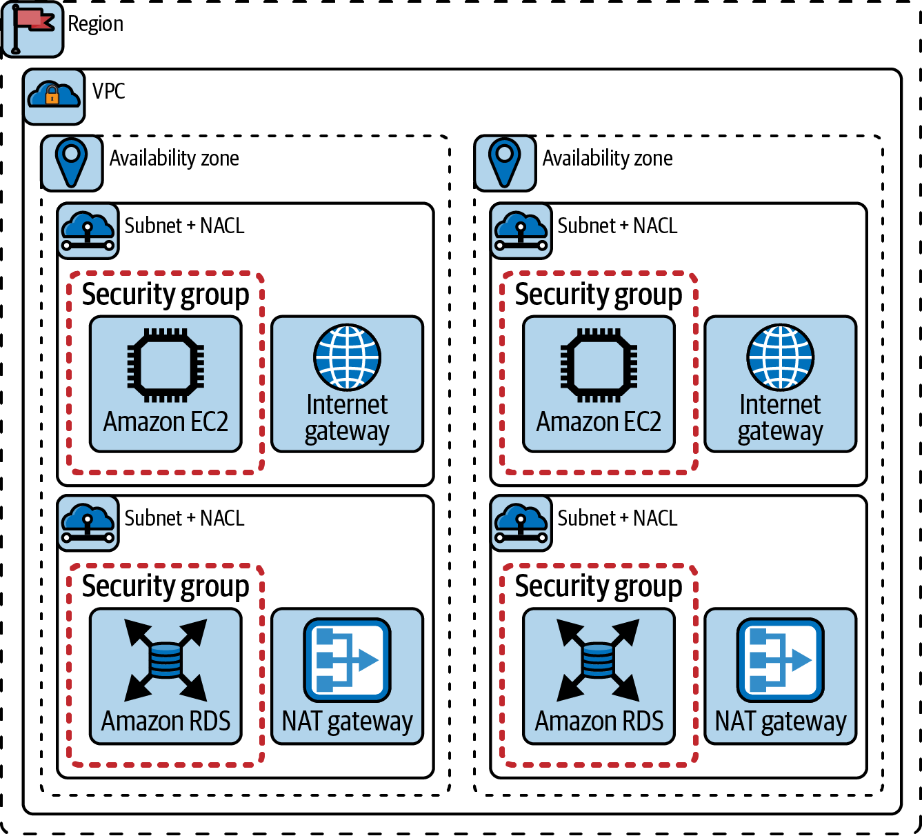
Figure 4-1. Single AWS VPC network topology
All of these things could be created manually and linked together using the AWS Management Console, but the opportunity for the network engineer here is to automate this process by using IaC tooling and processes. In “Network Automation in the Cloud”, we discuss the available programmable options for managing cloud resources.
A medium cloud network topology
Although a single VPC is very scalable, there are reasons to use multiple VPCs. The most obvious reason is that a VPC cannot span an AWS region; each VPC is limited to the region in which it was created. If you need to architect a network topology that can accommodate workloads in multiple regions, you’re looking at a multi-VPC topology. There are also other reasons for using multiple VPCs; just because you can put thousands of workloads in a single VPC doesn’t necessarily mean you should.
Public cloud providers design their infrastructure to be highly resilient and express this in the form of availability and durability SLAs. To go above these service offerings, you have to create your own high-availability architectures in the same way we do in on-premises data centers.
As soon as your topology goes to multiple VPCs, new challenges arise for the network engineer:
- Managing the IP address space
-
While each VPC can have identical, overlapping CIDR blocks, as soon as you want to connect VPCs together, you need to have nonoverlapping CIDR blocks. It’s necessary to architect a plan for how IP addresses will be carved out and allocated to VPCs in multiple regions while still planning for future growth (in terms of future subnets in existing VPCs, additional VPCs in current regions, and new VPCs in entirely new regions).
- Connectivity
-
AWS provides a way to connect VPCs together via VPC peering. VPC peering provides nontransitive connectivity between two VPCs and requires that VPC route tables are explicitly updated with routes to peer VPCs. When the number of VPCs is small, using VPC peering is manageable, but as the number of VPCs grows, the number of connections—and the number of route tables to be updated and maintained—also grows.
- Usage-based pricing
-
Although as a network engineer you can architect a topology that will provide the necessary connectivity among all the workloads in all the VPCs in all the regions, will your topology provide that connectivity in the most cost-effective way when usage increases? This means considering cross-AZ traffic charges, cross-region traffic charges, and egress charges to internet-based destinations (just to name a few).
All of these considerations layer on top of what’s already needed for smaller (single VPC) cloud network topologies.
A large cloud network topology
In a large cloud network topology, you’re looking at multiple dozens of VPCs in multiple regions worldwide. VPC peering is no longer a serviceable option; there are simply too many peering connections to manage, and nontransitive connectivity is introducing even more complexity.
A new set of design considerations emerge:
- Centralized connectivity
-
Using tools like transit VPCs and transit gateways, you can move away from the nontransitive VPC peering connectivity to a fully routed solution. These tools also allow you to integrate additional options like AWS Direct Connect (for dedicated connectivity back to on-premises networks) or VPN capabilities. Implementing centralized egress—where “spoke” VPCs use NAT gateways in the “hub” VPC for internet connectivity—is also possible. In all these cases, you need to define a routing strategy such as static routing or a dynamic routing protocol like BGP.
- Multi-account architectures
-
In topologies this large, you’re far more likely to encounter situations where entire VPCs belong to different AWS accounts. Your network topology now needs to address how to provide connectivity securely among resources that are owned by different entities.
Using the mentioned centralized connectivity tools, we can expand cloud networks to reach other cloud providers and on-premises networks.
A hybrid cloud network topology
With the increase in cloud service adoption, new interconnection scenarios are becoming more and more common. These scenarios include connecting different cloud providers (public or private) and connecting these cloud providers to on-premises networks; Flexera’s 2023 State of the Cloud Report says that 87% of the organizations surveyed use more than one cloud provider. Also, the boundaries between these environments are getting fuzzier, because cloud services can be running on their client’s on-premise data centers (for instance, AWS Outposts service). The industry uses the term hybrid cloud to describe these scenarios.
Aside from the challenges of managing and orchestrating various infrastructure services (and the applications on top), the first obvious challenge is how to connect all these environments together.
Hybrid cloud connectivity has no one-size-fits-all solution. All the public cloud service providers offer mechanisms to connect their services to on-premises networks. These mechanisms are usually based on VPN connections or dedicated connectivity services (e.g., AWS Direct Connect or Azure ExpressRoute). Figure 4-2 shows an example of a hybrid cloud network topology: an on-premises network is connected to AWS and Azure clouds via dedicated transport services, and the routing information is exchanged via BGP. Notice that you could also connect both cloud providers via the on-premises network.
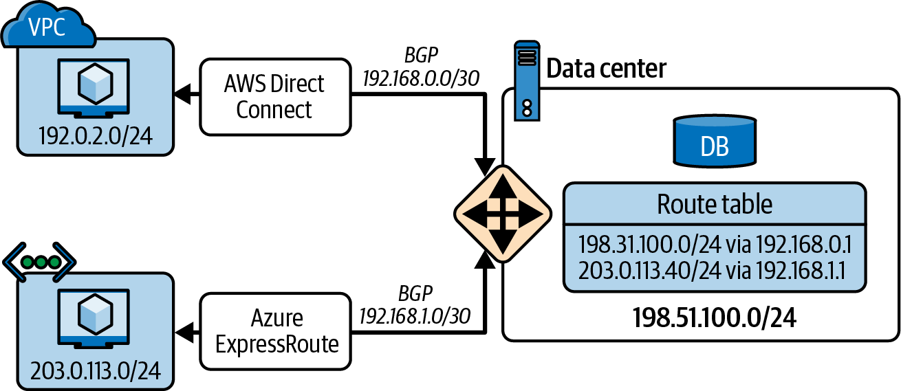
Figure 4-2. Hybrid network topology
Note
When you connect your network to a cloud provider, you can reach your own cloud workloads (e.g., your databases and VMs) but also the general cloud services. In the case of AWS, you can reach the object storage system Amazon Simple Storage Service (S3) and many more.
However, these connectivity mechanisms are not capable of directly interconnecting cloud providers. To interconnect cloud providers, you need to use other solutions such as routing them via an on-premises network as described in Figure 4-2 or creating your own VPN connections among the cloud providers to create an overlay network. If managing this interconnection becomes cumbersome, you can leverage third-party vendors that orchestrate these connections for you. Two examples of these vendors are Aviatrix and Alkira.
Either way, you still need to design a network topology that allows connecting all these environments, with a consistent network addressing and routing plan between network segments. This requires the network skills you have developed in your network engineering career.
Moreover, as the level of complexity grows, the need for automation increases exponentially. There are more “things” to manage and configure—things like transit gateway attachments, VPN connections, or separate subnets for certain types of connections. Managing them effectively will require some form of automation.
Network Automation in the Cloud
Networking in the cloud, unlike a lot of on-premises networking, is inherently built for automation. It’s a by-product of the qualities of cloud computing per the NIST definition provided in “Brief Definition of Cloud Computing”. We can approach network automation in the cloud in three ways:
-
Using the cloud provider’s APIs directly
-
Using the cloud provider’s CLI tool
-
Using a tool purpose-built for automating the cloud
Using the cloud provider’s APIs
Cloud providers offer API-first platforms. They have a rich set of APIs that can be used to automate the provisioning of cloud resources. Every other method (i.e., CLI tools or purpose-built tools) is just a wrapper around these APIs.
However, you won’t usually use the APIs directly. Even when you want to hit the APIs directly, you will likely use a programming language implementing a wrapper around the API (i.e., software development kit, or SDK). For instance, AWS maintains many SDKs for various programming languages, such as Boto3 for Python and AWS SDK for Go. Using an SDK makes API interaction easier because you don’t have to worry about the HTTP requests and responses.
Tip
The APIs support different versions to maintain backward compatibility in your code. The same applies to the SDKs.
In the following chapters, you will learn about programming languages (Chapters 6 and 7) as well as about HTTP APIs (Chapter 10). Therefore, we won’t cover examples of using the APIs here. You will find examples of using REST APIs, such as the ones exposed by AWS, in Chapter 10. There, you will learn about interacting with the APIs with various methods such as cURL, Postman, Python, and Go. Even though those examples are not specific to cloud service provisioning, all the APIs share the same principles so you can apply the knowledge to the cloud service provisioning use case.
Using the cloud provider’s CLI tool
The command-line interface is another UI to interact with the cloud provider’s APIs. The CLI tool offered by many of these cloud providers is often just a wrapper around that provider’s standard APIs, making it easier to interact with them. For instance, the AWS CLI tool leverages a Python SDK to expose this UI.
The CLI tool can be used manually by an operator to manage the cloud services, or it can be used in an automated fashion. For instance, you can use the CLI tool in a shell script. In Chapter 12, you will find examples (with the necessary configuration) of using the AWS CLI tool to interact with the AWS cloud. In the meantime, we give you an example from the AWS CLI repository of how to use the AWS CLI tool to create a VPC:
$ aws ec2 create-vpc \--cidr-block 10.0.0.0/16 \--tag-specification ResourceType=vpc,Tags=[{Key=Name,Value=MyVpc}]`{"Vpc": { "CidrBlock": "10.0.0.0/16", "DhcpOptionsId": "dopt-5EXAMPLE", "State": "pending", "VpcId": "vpc-0a60eb65b4EXAMPLE", "OwnerId": "123456789012", "InstanceTenancy": "default", "Ipv6CidrBlockAssociationSet": [], "CidrBlockAssociationSet": [ { "AssociationId": "vpc-cidr-assoc-07501b79ecEXAMPLE", "CidrBlock": "10.0.0.0/16", "CidrBlockState": { "State": "associated" } } ], "IsDefault": false, "Tags": [ { "Key": "Name", "Value": MyVpc" } ] } }

aws ec2 create-vpcis the command to create a VPC;ec2is the AWS service type, andcreate-vpcis the specific action.
Every AWS resource has mandatory and optional arguments. For the VPC, only the CIDR block is mandatory.

Tags, or metadata, is a common parameter for all cloud resources to add more dimensions to improve the resource classification.
The output of the command is a JSON object with the details of the created VPC, directly taken from the AWS API response.
You can find the complete AWS CLI tool documentation online.
Using a tool purpose-built for automating the cloud
On top of the cloud provider’s APIs, purpose-built tools have been built to automate the cloud. These tools are usually called infrastructure as code tools because they allow you to define your infrastructure as code (in a declarative approach) and then manage it accordingly.
You could also automate the cloud by using an imperative approach (e.g., using Ansible), but we consider that an antipattern for service provisioning, so we recommend it for configuration management. Both approaches can coexist, as you may need to configure some services after provisioning them. We take a deep dive into this topic in Chapter 12.
To classify the tools implementing a declarative approach, we have to consider two dimensions: whether they are cloud-specific or multicloud, and whether they use a programming language or a domain-specific language (DSL) to define the infrastructure.
Note
A DSL is designed to solve a specific problem; in contrast, a programming language is a general-purpose language that can be used to solve any problem. DSLs are intended to be used by nonprogrammers, so they are usually easier to learn and use than programming languages, but they are less flexible. Examples of DSLs are Structured Query Language (SQL), HTML, the YAML-based syntax used in Ansible playbooks, and HashiCorp Configuration Language (HCL) used in Terraform (more about YAML in Chapter 8 and about Ansible and HCL/Terraform in Chapter 12).
In Table 4-1, we use these two dimensions to classify a few of the most popular tools.
| Programming language | Domain-specific language | |
|---|---|---|
Single cloud |
AWS Cloud Development Kit (CDK) |
AWS CloudFormation, Azure Resource Manager |
Multicloud |
Pulumi, CDK for Terraform |
Terraform |
You should choose the most appropriate tool for your context. In Chapter 12, we explain how to use Terraform and its DSL, because it’s the most popular tool for multicloud environments.
After this brief introduction to cloud networking, we will now move on to discuss the relationship between containers and cloud services.
Containers
Unless you haven’t been paying attention to what’s happening in the technology world, you almost surely have heard of containers. Containers are, in the end, just processes running on an OS instance. In fact, a key facet to understanding containers is that there is no such thing as a container. What we refer to as a container is a process running on an OS instance that may or may not take advantage of certain OS features. So why are containers getting so much attention? There are some very good reasons:
- Isolation
-
A process running in a container—or you could say a containerized process—is isolated from other processes by a series of OS-level features called namespaces. These namespaces can isolate the process in a variety of ways; for example, the process can be made to think it’s the only process running on the OS (via the “process identifier,” or PID namespace), that it has its own network interfaces (via the network namespace), or that it has its own set of users and groups (via the user namespace). The exact set of namespaces employed will vary based on the container runtime (the engine responsible for setting up processes to run in a container), the presence or absence of a container orchestrator (a tool responsible for managing the lifecycle of containers), and other factors. You’ll see this in action in the section on Kubernetes, a popular container orchestration platform.
- Distribution
-
Another aspect of containers is that they are built from a container image. A container image bundles together all the dependencies needed by the process that will run in a container; this includes any executables, system libraries, tools, or even environment variables and other required configuration settings. Because a container image doesn’t include the full kernel and OS—it contains what is needed to run only one specific process—images are typically much smaller than a VM image. When coupled with the ability for image creators to easily publish (push) container images to a registry, and for other users to easily retrieve (pull) images from a registry, it becomes easy to widely distribute container images.
Consider an open source project like the Caddy web server. The maintainers of a project like Caddy can bundle their project and all its dependencies and provide that in a container image for users. Users can pull the Caddy container image and deploy it in a few minutes with a couple of commands.
- Reuse
-
Not only are container images easy to build, easy to distribute, and easy to consume, but they are also easy for others to reuse. Consider again the Caddy web server. If a user wants to deploy Caddy along with custom web content, it’s trivial to build a new container image based on the Caddy container image. Someone else could, in turn, reuse your custom image to build their own custom image. Arguably, this ease of reuse could be one of the most important and influential aspects of containers and container images.
- Speed
-
A container doesn’t run any faster than a “normal” process on a host, but containers themselves are far faster to start than other isolation mechanisms, like VMs. The size of a container image—sometimes as low as tens of megabytes in size, compared to hundreds or thousands of megabytes for a VM disk image—makes containers faster to distribute. Finally, new container images can often be built in minutes, making the time investment for creating a new container image significantly lower than the time investment required to build a VM image, even when using VM image creation automation tools like Packer.
Containers became popular in 2013 with the introduction of Docker, but containers have been around for far longer than that. Before Docker’s arrival, containers existed in the form of LXC, Linux-VServer, OpenVZ, FreeBSD jails, Oracle Solaris Containers (and Solaris Zones), and even going all the way back to the original introduction of chroot. All of these were OS-level mechanisms for isolating processes running on a host. LXC is considered the first complete implementation of containers that leveraged both control groups (cgroups) for limiting resource utilization and namespaces for isolating processes without the need for a custom Linux kernel.
Note
If you’re interested in more details on Docker, we recommend Using Docker by Adrian Mouat (O’Reilly).
Following the rise of Docker, standards around containers began to emerge. One key standardization effort is the Open Container Initiative, or OCI, which was formed in 2015 by Docker, CoreOS (now part of Red Hat, which in turn is part of IBM), and others. OCI helped establish standards around the image specification (how container images are built), the runtime specification (how a container is instantiated from a container image), and the distribution specification (how containers are distributed and shared via a registry). Driven in part by this standardization (and to some extent helping to drive this standardization), standard implementations also began to emerge: runc as a standard implementation of running a container according to the OCI specification, and containerd as a standard implementation of a full-lifecycle container runtime that builds on top of runc.
Note
Although great strides have been made in recent years in adding containerization functionality to Windows, containers remain—even today—largely a Linux-only thing. Throughout the discussion of containers in this chapter, the focus is only on Linux containers.
Now that you have a better understanding of what containers are and what benefits they offer, let’s answer the question of why we are discussing containers in a cloud-focused chapter, especially when you’ve already seen that containers are predominantly a Linux-focused entity. Why not put them in the Linux chapter, instead of the cloud chapter?
What Do Containers Have to Do with the Cloud?
In and of themselves, containers have nothing to do with cloud computing. They are an OS-level construct and are equally at home on your local laptop, on a VM running on a hypervisor in a data center, or on a cloud instance. Since their introduction, however, containers have grown to be a key part of cloud native computing. As defined by the Cloud Native Computing Foundation (CNCF), cloud-native computing enables “organizations to build and run scalable applications in modern and dynamic environments such as public, private, and hybrid clouds, while leveraging cloud computing benefits to their fullest.”
Given the importance of containers to cloud native computing, and given the prevalence of container-based services offered by public cloud providers today—like AWS ECS, Google Cloud Run, and Azure Container Instances (ACI)—we feel the placement of containers in this cloud chapter is appropriate.
What Do Containers Have to Do with Networking?
The placement of containers within a cloud-focused chapter hopefully makes sense, but a larger question still needs answering: what do containers have to do with networking? We feel it’s important to include content on containers in a networking programmability and automation book for a few reasons:
-
The way in which container networking is handled—especially when containers are used in conjunction with the Kubernetes container orchestration platform—is sufficiently different from what most network engineers already know and understand that it’s worth highlighting these differences and building a bridge between Kubernetes concepts and more “typical” networking constructs.
-
Network engineers may wish to use containers in conjunction with other tools. A network engineer might, for example, want to create a “network tools” container image that has all of the most important networking and network automation tools (including all necessary dependencies) bundled into a single image that is easily distributed and executed on any compatible platform. Containers also simplify spinning up network development environments, as you will learn in Chapter 5 when we cover Containerlab.
-
Network vendors may leverage containers in their platforms, especially on Linux-based platforms. The isolation mechanisms of containers combined with the ease of distribution make containers an ideal method for delivering new functionality to networking platforms.
So, we’ll review the basics of container networking, including how containers are isolated from one another, and how they can communicate with one another and with the outside world.
Extending Linux Networking for Containers
One reason the Linux chapter (Chapter 3) spends so much time on the basic building blocks of networking is that containers (and container orchestration systems like Kubernetes, as you’ll see in “Kubernetes”) extend these basic building blocks to accommodate container networking. A good understanding of the basic building blocks provides the necessary structure that makes it easier to add container-specific concepts to your skill set.
For networking containers, five Linux technologies are leveraged:
-
Network namespaces
-
Virtual Ethernet (veth) interfaces
-
Bridges
-
IP routing
-
IP masquerading
Of these, bridges and IP routing—a term used to describe the ability of a Linux-based system to act as a Layer 3 (IP-based) router—were discussed in Chapter 3. The remaining three technologies are discussed in the following sections. We start with Linux network namespaces.
Linux network namespaces
Namespaces are an isolation mechanism; they limit what processes can “see” in the namespace. The Linux kernel provides multiple namespaces; for networking, network namespaces are the primary namespaces involved. Network namespaces can be used to support multiple separate routing tables or multiple separate iptables configurations, or to scope, or limit, the visibility of network interfaces. In some respects, they are probably most closely related to VRF instances in the networking world.
Note
While network namespaces can be used to create VRF instances, separate work is going on in the Linux kernel community right now to build “proper” VRF functionality into Linux. This proposed VRF functionality would provide additional logical Layer 3 separation within a namespace. It’s still too early to see where this will lead, but we want you to know about it nevertheless.
Some use cases for Linux network namespaces include the following:
- Per-process routing
-
Running a process in its own network namespace allows you to configure routing per process.
- Enabling VRF configurations
-
We mentioned at the start of this section that network namespaces are probably most closely related to VRF instances in the networking world, so it’s only natural that enabling VRF-like configurations would be a prime use case for network namespaces.
- Support for overlapping IP address spaces
-
You might also use network namespaces to provide support for overlapping IP address spaces, where the same address (or address range) might be used for different purposes and have different meanings. In the bigger picture, you’d probably need to combine this with overlay networking and/or NAT in order to fully support such a use case.
- Container networking
-
Network namespaces are also a key part of the way containers are connected to a network. Container runtimes use network namespaces to limit the network interfaces and routing tables that the containerized process is allowed to see or use.
In this discussion of network namespaces, the focus is on that last use case—container networking—and how network namespaces are used. The focus is further constrained to discuss only how the Docker container runtime uses network namespaces. Finally, as mentioned earlier, we will discuss only Linux containers, not containers on other OSs.
In general, when you run a container, Docker will create a network namespace for that container. You can observe this behavior by using the lsns command. For example, if you run lsns -t net to show the network namespaces on an Ubuntu Linux system that doesn’t have any containers running, you would see only a single network namespace listed.
However, if you launch a Docker container on that same system with docker run --name nginxtest -p 8080:80 -d nginx, then lsns -t net will show something different. Here’s the output of lsns -t net -J, which lists the network namespaces serialized as JSON:
{"namespaces":[{"ns":4026531840,"type":"net","nprocs":132,"pid":1,"user":"root","netnsid":"unassigned","nsfs":null,"command":"/sbin/init"},{"ns":4026532233,"type":"net","nprocs":5,"pid":15422,"user":"root","netnsid":"0","nsfs":"/run/docker/netns/b87b15b217e8","command":"nginx: master process nginx -g daemon off;"}]}
The host (or root, or default) namespace that is present on every Linux system. When we interact with network interfaces, routing tables, or other network configurations, we are generally interacting with the default namespace.
The namespace created by Docker when we ran (created) the container. There are multiple ways to determine that this is the namespace Docker created, but in this case looking at the
commandfield gives it away.
In some cases—like the preceding example—it’s easy to tell which network namespace is which. For a more concrete determination, you can use the following steps:
-
Use the
docker container lscommand to get the container ID for the container in question. -
Use the
docker container inspect container-idcommand to have the Docker runtime provide detailed information about the specified container. This will produce a lot of output in JSON; you may find it easier to deal with this information if you pipe it through a utility likejq. -
Look for the
SandboxKeyproperty. It will specify a path, like/var/run/docker/netns/b87b15b217e8. Compare that with the output oflsnsand itsnsfsproperty. With the exception of the/varprefix, the values will match when you are looking at the same container.
Note
If you don’t want to run a container in a network namespace, Docker supports a --network=host flag that will launch the container in the host (also known as the root, or default) namespace.
The ip command (from the iproute2 package), which Chapter 3 covers in great detail, also has an ip netns subcommand that allows the user to create, manipulate, and delete network namespaces. However, the network namespaces created by Docker and other container runtimes generally aren’t visible to the user, even if used with sudo to gain elevated permissions. The lsns command used in this section, however, will show network namespaces created by Docker or another container runtime. (Although we are discussing only network namespaces here, lsns can show any type of namespace, not just network namespaces.)
Network namespaces have more use cases than just containers; for a more detailed look at working with network namespaces in a noncontainer use case, refer to the additional online content for this book. There you’ll find examples of how to use the ip netns command to manipulate the networking configuration of a Linux host, including adding interfaces to and removing interfaces from a network namespace.
Linux network namespaces are a critical component for container networking, but without a mechanism for simulating the behavior of a real network interface, our systems’ ability to connect containers to the network would be greatly constrained. In fact, we’d be able to run only as many containers as we could fit physical network interfaces in the host. Virtual Ethernet interfaces are the solution to that constraint.
Virtual Ethernet interfaces
Just as network namespaces enable the Linux kernel to provide network isolation, Virtual Ethernet (also called veth) interfaces enable you to intentionally break that isolation. Veth interfaces are logical interfaces; they don’t correspond to a physical NIC or other piece of hardware. As such, you can have many more veth interfaces than you have physical interfaces.
Further, veth interfaces always come in pairs: traffic entering one interface in the pair comes out the other interface in the pair. For this reason, you may see them referenced as veth pairs. Like other types of network interfaces, a veth interface can be assigned to a network namespace. When a veth interface—one member of a veth pair—is assigned to a network interface, you’ve just connected two network namespaces to each other (because traffic entering a veth interface in one namespace will exit the other veth interface in the other namespace).
This underlying behavior—placing one member of a veth pair in a network namespace and leaving the peer interface in the host (or default) namespace—is the key to container networking. This is how all basic container networking works.
Using the same Docker container spun up in the previous section (which was a simple nginx container launched with the command docker run --name nginxtest -p 8080:80 -d nginx), let’s look at how this container’s networking is handled.
First, you already know the network namespace the nginx container is using; you determined that using lsns -t net along with docker container inspect and matching up the nsfs and SandboxKey properties from each command, respectively.
Using this information, you can now use the nsenter command to run other commands within the namespace of the nginx Docker container. (For full details on the nsenter command, use man nsenter.) The nsenter flag to run a command in the network namespace of another process is -n, or --net, and it’s with that flag you’ll provide the network namespace for the nginx container as shown in Example 4-1.
Example 4-1. Running ip link within a namespace with nsenter
ubuntu2004:~$ sudo nsenter --net=/run/docker/netns/b87b15b217e8 ip link list
1: lo: LOOPBACK,UP,LOWER_UP mtu 65536 qdisc noqueue state UNKNOWN mode DEFAULT
 group default qlen 1000
    link/loopback 00:00:00:00:00:00 brd 00:00:00:00:00:00
4: eth0@if5: BROADCAST,MULTICAST,UP,LOWER_UP mtu 1500 qdisc noqueue state UP
 mode DEFAULT group default
    link/ether 02:42:ac:11:00:02 brd ff:ff:ff:ff:ff:ff link-netnsid 0
The interface name is
eth0@if5. The interface index—the number at the beginning of the line before the interface name—is4.
Compare that with the output of ip link list in the host (default) network namespace from Example 4-2.
Example 4-2. Running ip link in the host network namespace
ubuntu2004:~$iplinklist1:lo:LOOPBACK,UP,LOWER_UPmtu65536qdiscnoqueuestateUNKNOWNmodeDEFAULTgroupdefaultqlen1000link/loopback00:00:00:00:00:00brd00:00:00:00:00:002:ens5:BROADCAST,MULTICAST,UP,LOWER_UPmtu9001qdiscmqstateUPmodeDEFAULTgroupdefaultqlen1000link/ether02:95:46:0b:0f:ffbrdff:ff:ff:ff:ff:ffaltnameenp0s53:docker0:BROADCAST,MULTICAST,UP,LOWER_UPmtu1500qdiscnoqueuestateUPmodeDEFAULTgroupdefaultlink/ether02:42:70:88:b6:77brdff:ff:ff:ff:ff:ff5:veth68bba38@if4:BROADCAST,MULTICAST,UP,LOWER_UPmtu1500qdiscnoqueuemasterdocker0stateUPmodeDEFAULTgroupdefaultlink/ethera6:e9:87:46:e7:45brdff:ff:ff:ff:ff:fflink-netnsid0
The interface with
vethin the name is one indicator that this might be a veth interface. Names can be changed, though, so this is not a foolproof indicator. However, the name showsveth68bba38@if4, and the interface index is5.
The connection between both outputs is the @ifX suffix. On the interface with the index of 5 (that’s the veth68bba38 interface in the host namespace), the suffix points to the interface whose index is 4. The interface with the index of 4 is eth0 in the nginx container’s network namespace (see Example 4-1), and its suffix points to interface index 5 (see Example 4-2).
This is how you can determine veth pairs, and in this case, you see that Docker has created a veth pair for this container. One member of the veth pair is placed in the nginx container’s network namespace, and the other member of the veth pair remains in the host namespace. In this configuration, traffic that enters eth0@if5 in the nginx container’s network namespace will exit veth68bba38@if4 in the host namespace, thus traversing from one namespace to another namespace.
Tip
You can also use ip -d link list to show more details in the output. The additional output will include a line with the word veth to denote a member of a veth pair. This command will also clearly indicate when an interface is a bridge interface (the additional output will show bridge) as well as when an interface is part of a bridge (denoted by bridge_slave). Also, in the event the @ifX suffix isn’t present, you can use ethtool -S veth-interface, which will include the line peer_ifindex: in the output. The number there refers to the interface index of the other member of the veth pair.
Veth interfaces enable container traffic to move from its own network namespace to the host network namespace (assuming that the container was not started with the --network=host flag), but how does traffic get from the veth interface in the host namespace onto the physical network? If you guess a bridge, you guessed correctly! (To be fair, bridges were listed at the beginning of this section as a component of container networking.)
The key in Example 4-2, as discussed in “Bridging (Switching)”, is the appearance of master docker0 related to veth68bba38@if4. The presence of this text indicates that the specified interface is a member of the docker0 Linux bridge. If you examine the rest of the interfaces, however, you’ll note that none of them is a member of the docker0 bridge. How, then, does the traffic actually get onto the physical network? This is where IP masquerading comes in, which is the final piece in the puzzle of how Docker containers on a Linux host connect to a network.
Note
Veth interfaces have more uses, although most involve connecting network namespaces together. Refer to the extra online content for this book for additional examples of using veth interfaces, as well as a look at the commands for creating, modifying, and removing veth interfaces.
IP masquerading
In exploring container networking, so far you’ve seen how container runtimes like Docker use network namespaces to provide isolation—preventing a process in one container from having any access to the network information of another container or of the host. You’ve also seen how veth interfaces (also referred to as veth pairs) are used to connect the network namespace of a container to the host network namespace. Building upon the extensive coverage of interfaces, bridging, and routing from Chapter 3, you’ve also seen how a Linux bridge is used in conjunction with the veth interfaces in the host namespace. Only one piece remains: getting the container traffic out of the host and onto the network. This is where IP masquerading gets involved.
IP masquerading enables Linux to be configured to perform NAT. NAT, as you’re probably aware, allows one or more computers to connect to a network by using a different address. In the case of IP masquerading, one or more computers connect to a network by using the Linux server’s own IP address. RFC 2663 refers to this form of NAT as network address port translation (NAPT); it’s also referred to as one-to-many NAT, many-to-one NAT, port address translation (PAT), and NAT overload.
Before going much further, it’s worth noting here that Docker supports several types of networking:
- Bridge
-
This is the default type of networking. It uses veth interfaces, a Linux bridge, and IP masquerading to connect containers to physical networks.
- Host
-
When using host mode networking, the Docker container is not isolated in its own network namespace; instead, it uses the host (default) network namespace. Exposed ports from the container are available on the host’s IP address.
- Overlay
-
Overlay networking creates a distributed network spanning multiple Docker hosts. The overlay networks are built using VXLAN, defined in RFC 7348. This mode of networking is directly tied to Docker’s container orchestration mechanism, called Swarm.
- IPvlan and macvlan
-
IPvlan networking allows multiple IP addresses to share the same MAC address of an interface, whereas macvlan networking assigns multiple MAC addresses to an interface. The latter, in particular, does not generally work on cloud provider networks. Both IPvlan and macvlan networking are less common than other network types.
Tip
Macvlan networking using macvlan interfaces can be used for other purposes besides container networking. More information on macvlan interfaces and macvlan networking is found at the extra online content for this book.
Throughout this section on container networking, the discussion has centered on bridge mode networking with Docker.
When using bridge mode networking with Docker, the container runtime uses a network namespace to isolate the container and a veth pair to connect the container’s network namespace to the host namespace. In the host namespace, one of the veth interfaces is attached to a Linux bridge. If you launch more containers on the same Docker network, they’ll be attached to the same Linux bridge, and you’ll have immediate container-to-container connectivity on the same Docker host. So far, so good.
When a container attempts to connect to something that’s not on the same Docker network, Docker has already configured an IP masquerading rule that will instruct the Linux kernel to perform many-to-one NAT for all the containers on that Docker network. This rule is created when the Docker network is created. Docker creates a default network when it is installed, and you can create additional networks by using the docker network create command.
First, let’s take a look at the default Docker network. Running docker network ls shows a list of the created Docker networks. On a freshly installed system, only three networks will be listed (the network IDs listed will vary):
ubuntu2004:~$dockernetworklsNETWORKIDNAMEDRIVERSCOPEb4e8ea1af51bbridgebridgelocaladd089049cdahosthostlocalfbe6029ce9f7nonenulllocal
Using the docker network inspect command displays full details about the specified network. Here’s the output of docker network inspect b4e8ea1af51b showing more information about the default bridge network (some fields were omitted or removed for brevity):
[{"Name":"bridge","Id":"b4e8ea1af51ba023a8be9a09f633b316f901f1865d37f69855be847124cb3f7c","Created":"2023-04-16T18:27:14.865595005Z","Scope":"local","Driver":"bridge","EnableIPv6":false,"IPAM":{"Driver":"default","Options":null,"Config":[{"Subnet":"172.17.0.0/16"}]},"Options":{"com.docker.network.bridge.default_bridge":"true","com.docker.network.bridge.enable_icc":"true","com.docker.network.bridge.enable_ip_masquerade":"true","com.docker.network.bridge.host_binding_ipv4":"0.0.0.0","com.docker.network.bridge.name":"docker0","com.docker.network.driver.mtu":"1500"},"Labels":{}#outputomittedforbrevity}]
The subnet used by containers is
172.17.0.0/16.Docker will automatically create the necessary IP masquerading rules for this network.
The name of the bridge for this network is
docker0(shown in theOptionssection).
You can verify this information by using Linux networking commands covered in Chapter 3 and in this section. For example, to see the IP address assigned to the nginx Docker container launched earlier, you use a combination of nsenter and ip addr list, like this:
ubuntu2004:~$ sudo nsenter --net=/run/docker/netns/b87b15b217e8 ip addr list eth0
4: eth0@if5: BROADCAST,MULTICAST,UP,LOWER_UP mtu 1500 qdisc noqueue state UP
 group default
    link/ether 02:42:ac:11:00:02 brd ff:ff:ff:ff:ff:ff link-netnsid 0
    inet 172.17.0.2/16 brd 172.17.255.255 scope global eth0
       valid_lft forever preferred_lft forever
Verifies that the container is using an address from the
172.17.0.0/16network
Similarly, running ip -br link list (the -br flag stands for brief and displays abbreviated output) shows that the bridge created by Docker is indeed named docker0:
ubuntu2004:~$ ip -br link list
lo               UNKNOWN  00:00:00:00:00:00 LOOPBACK,UP,LOWER_UP
ens5             UP       02:95:46:0b:0f:ff BROADCAST,MULTICAST,UP,LOWER_UP
docker0          UP       02:42:70:88:b6:77 BROADCAST,MULTICAST,UP,LOWER_UP
veth68bba38@if4  UP       a6:e9:87:46:e7:45 BROADCAST,MULTICAST,UP,LOWER_UP
The last piece is the IP masquerading rule, which you can verify by using the iptables command. Using iptables is a topic that could have its own book, and does, in fact—see Linux iptables Pocket Reference by Gregor N. Purdy (O’Reilly). We can’t cover it in great detail but can provide a high-level overview and then explain where the Docker IP masquerading rule fits in.
Note
Technically, iptables has been replaced by nftables. However, the Linux community still largely references iptables, even when referring to nftables. Additionally, the iptables command (and its syntax) continues to work even though the underlying mechanism is now nftables.
Iptables provides several tables, like the filter table, the NAT table, and the mangle table. Additionally, there are multiple chains, like PREROUTING, INPUT, OUTPUT, FORWARD, and POSTROUTING. Each chain is a list of rules, and not every table will have every chain. The rules in a chain match traffic based on properties like source address, destination address, protocol, source port, or destination port. Each rule specifies a target, like ACCEPT, DROP, or REJECT.
With this additional information in hand, let’s look at the iptables command. In Example 4-3, we use this command to show you all the chains and rules in the NAT table.
Example 4-3. Listing all chains and rules in the NAT table with iptables
ubuntu2004:~$ iptables -t nat -L -n
The
-t natparameter tellsiptablesto display the NAT table. The-Llists the rules, and-nsimply instructsiptablesto show numbers instead of attempting to resolve them into names.The rule specifies the source as
172.17.0.0/16. We know that to be the subnet assigned to the default Docker bridge network.The rule specifies a destination of
0.0.0.0/0(anywhere).The target for traffic that matches the rule is
MASQUERADE. This target is available only in the NAT table and in thePOSTROUTINGchain.
By the time traffic hits the POSTROUTING chain in the NAT table, routing has already been determined (for more details on how Linux routing works, see “Routing as an End Host” and “Routing as a Router”), and the outbound interface has already been selected based on the host’s routing configuration. The MASQUERADE target instructs iptables to use the IP address of the outbound interface as the address for the traffic that matches the rule—in this case, traffic from the Docker network’s subnet bound for anywhere. This is how, when using a Docker bridge network, traffic actually makes it onto the network: the Linux host determines a route and outbound interface based on its routing table and sends the Docker container traffic to that interface. The rule in the POSTROUTING chain of the NAT table grabs that traffic and performs many-to-one NAT using the selected interface’s IP address.
Many Linux distributions also provide an iptables-save command, which shows the iptables rules in a slightly different format. This is how iptables-save shows the rule created by Docker for masquerading a bridge network:
ubuntu2004:~$ sudo iptables-save -t nat
...output omitted...
-A POSTROUTING -s 172.17.0.0/16 ! -o docker0 -j MASQUERADE
...output omitted...
In this format, you can clearly see the specified source (-s 172.17.0.0/16), and the ! -o docker0 is shorthand indicating that the outbound interface is not the docker0 bridge. In other words, traffic coming from 172.17.0.0/16 is not bound for any destination on the docker0 bridge. The target is specified by -j MASQUERADE.
Before moving on to the next section, we present a visual summary of the previous examples in Figure 4-3. You can observe the container running on a network namespace (other namespaces may exist in the same host) that is connected to the default (host) namespace via a veth interface. The veth interface is connected to the docker0 bridge, which is connected to the host’s physical interface, and finally, via IP masquerading, to the rest of the network.
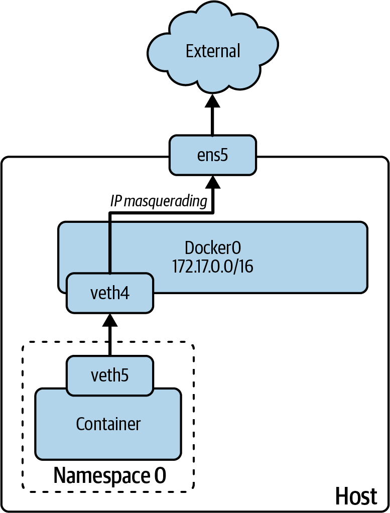
Figure 4-3. Container networking summary
It’s now time to transition to Kubernetes, a popular container orchestration tool. Although many of the concepts introduced in this section still apply—Kubernetes is working with containers, after all—a few notable differences exist. The next section touches on those differences and builds on what you already know about container networking.
Kubernetes
Although not necessarily strictly tied to cloud computing—one could make the argument that Kubernetes is a form of PaaS—the use of cloud native to describe Kubernetes has inevitably and deeply linked this successful open source project with cloud computing. You’ve already seen how containers themselves are associated with cloud computing; it’s only natural that the position of Kubernetes in the realm of cloud computing is further solidified by the fact that it is a container orchestrator and is responsible for orchestrating the lifecycle of containers across a fleet of compute instances.
Finally, the predecessors to Kubernetes were systems internal to Google—Borg and later Omega—that were responsible for managing the compute capacity across thousands of nodes. Kubernetes was, truly, “born from the cloud.”
Note
Kubernetes is not the only container orchestrator but is the most popular. Other container orchestrators include Nomad and Docker Swarm. Many other container orchestration platforms are built on top of Kubernetes, such as OpenShift and Rancher by SUSE.
Before discussing networking in Kubernetes, it’s important to explain some of the key concepts found in Kubernetes, along with important terminology.
Key Kubernetes Concepts
Kubernetes is, at the core, a distributed system responsible for managing compute workloads across units of compute capacity. The “compute workloads” are containers, which is why Kubernetes is often referred to as a container orchestration platform. The “units of compute capacity” are referred to as nodes, and they can be bare-metal instances, cloud instances, or VMs running on an on-premises hypervisor like VMware vSphere.
Kubernetes nodes are organized into clusters. Each cluster has a control plane, running on one or more nodes, that provides the management functions for the cluster. Nodes that run the control plane components for the cluster are control plane nodes. Nodes that aren’t part of the control plane are worker nodes.
The control plane has three pieces: the API server, the controller manager, and the scheduler. Each performs a different but critical function in the overall operation of the Kubernetes cluster. The scheduler is responsible for placing workloads on worker nodes, while the API server exposes the control plane to users (and other systems). We’ll discuss the controller manager shortly.
Backing the control plane is a distributed key-value store named etcd; this typically runs on the control plane nodes but can run external to the cluster if desired. Etcd—which also forms clusters—needs to have an odd number of instances in order to establish and maintain quorum. Typically, you’ll see three etcd instances, along with three control plane instances, in a highly available Kubernetes cluster. It is possible, however, to run a Kubernetes cluster with a single etcd instance and a single control plane node.
Note
Although etcd has requirements about the number of instances to establish and maintain quorum, the Kubernetes control plane components themselves have no such requirements. You can run two control plane nodes for availability, if desired. However, etcd often runs on the control plane nodes themselves, and in that case, you’ll find three instances of the Kubernetes control plane components.
The Kubernetes API server implements a RESTful declarative API: users (and other systems) don’t use the Kubernetes API to tell the cluster what to do (an imperative approach), but rather to tell the cluster what the desired outcome is (a declarative approach). For example, using the API, you wouldn’t instruct a Kubernetes cluster to create three workloads. Instead, you would tell the Kubernetes cluster you want three workloads running, and you leave the “how” to the cluster itself.
This behavior is known as reconciliation of the desired state (the desired outcome you’ve given the cluster) against the actual state (what is actually running or not running on the cluster). This happens constantly within Kubernetes and is often referred to as the reconciliation loop. Reconciling the desired state against the actual state sits at the heart of everything Kubernetes does and the way Kubernetes operates.
Every action that’s taken in a Kubernetes cluster happens via the reconciliation loop. For every kind of API object that Kubernetes knows about, something has to implement the reconciliation loop. That “something” is known as a controller, and the controller manager—the third part of the Kubernetes control plane, along with the scheduler and the API server—is responsible for managing the controllers for the built-in objects that Kubernetes understands. New types of objects can be created, via a custom resource definition (CRD), but the new types of objects will also require a controller that understands the lifecycle of those objects: how they are created, how they are updated, and how they are deleted.
Tip
O’Reilly has published several books focused exclusively on Kubernetes that may be helpful. Titles to consider include Kubernetes: Up and Running, 3rd Edition, by Brendan Burns et al.; Kubernetes Cookbook by Sébastien Goasguen and Michael Hausenblas; Production Kubernetes by Josh Rosso et al.; and Kubernetes Patterns by Bilgin Ibryam and Roland Huß.
A lot more could be said about Kubernetes, but this basic introduction gives you enough information to understand the rest of this section. Next we discuss some of the basic building blocks involved in Kubernetes networking.
Building Blocks of Networking in Kubernetes
Kubernetes introduces a few new constructs, but it’s important to remember that Kubernetes is built on top of existing technologies. In the following sections, we discuss the basic building blocks of Kubernetes networking, and how they relate to the networking technologies you already know, such as container networking, IP routing, and load balancing, among others.
Pods
A Pod is a collection of containers that share network access and storage volumes. A Pod may have one container or multiple containers. Regardless of the number of containers within a Pod, however, certain things remain constant:
-
All the containers within a Pod are scheduled together, created together, and destroyed together. Pods are the atomic unit of scheduling.
-
All the containers within a Pod share the same network identity (IP address and hostname). Kubernetes accomplishes this by having multiple containers share the same network namespace—which means they share the same network configuration and the same network identity. This does introduce some limitations; for example, two containers in a Pod can’t expose the same port. The basics of how these containers connect to the outside world remain as described in “Containers”, with a few minor changes.
-
A Pod’s network identity (IP address and hostname) is ephemeral; it is allocated dynamically when the Pod is created and released when the Pod is destroyed or dies. As a result, you should never construct systems or architectures that rely on directly addressing Pods; after all, what will happen when you need to run multiple Pods? Or what happens when a Pod dies and gets re-created with a different network identity?
-
All the containers within a Pod share the same storage volumes and mounts. This is accomplished by having containers share the namespace responsible for managing volumes and mounts.
-
Kubernetes provides higher-level mechanisms for managing the lifecycle of Pods. For example, Deployments are used by Kubernetes to manage ReplicaSets, which in turn manage groups of Pods to ensure that the specified number of Pods is always running in the cluster.
To create a Pod, a cluster user or operator would typically use a YAML file that describes the Pod to the Kubernetes API server. The term given to these YAML files is manifests, and they are submitted to the API server (typically via the Kubernetes command-line tool, kubectl, or its equivalent). Example 4-4 shows a manifest for a simple Pod.
Example 4-4. Kubernetes Pod manifest
apiVersion:v1kind:Podmetadata:name:assetslabels:app.kubernetes.io/name:zephyrspec:containers:-name:assetsimage:nginxports:-name:http-altcontainerPort:8080protocol:TCP
The Kubernetes API supports versioning. When the API version is just
v1, as here, it means this object is part of the Kubernetes core API.kindrefers to Kubernetes construct types, like Pod, Deployment, Service, Ingress, NetworkPolicy, etc.Every API object also has metadata associated with it. Sometimes the metadata is just a name, but many times—as in this example—it also includes labels. Labels are heavily used throughout Kubernetes.
A Pod can have one or more containers. In this example, only a single container is in the Pod, but more items could be in the list.

The
imagespecified here is a container image. This container image will be used to create a new container in the Pod. In this example, only a single container is in the Pod.
Pods can expose one or more ports to the rest of the cluster.
When creating Pods, Kubernetes itself doesn’t create the containers; that task is left to the container runtime. Kubernetes interacts with the container runtime via a standard interface known as the Container Runtime Interface (CRI). Similar standard interfaces exist for storage (Container Storage Interface, or CSI) and networking (Container Network Interface, or CNI). CNI is an important part of Kubernetes networking, but before discussing CNI, let’s take a look at Kubernetes Services.
Services
If you can’t connect directly to a Pod, how can applications running in Pods possibly communicate across the network? This is one of the most significant departures of Kubernetes from previous networking models. When working with VMs, the VM’s network identity (IP address and/or hostname) is typically long-lived, and you can plan on being able to connect to the VM in order to access whatever applications might be running on that VM. As you shift into containers and Kubernetes, that’s no longer true. A Pod’s network identity is ephemeral. Further, what if there are multiple replicas of a Pod? To which Pod should another application or system connect?
Instead of connecting to a Pod (or to a group of Pods), Kubernetes uses a Service (Example 4-5 shows a manifest for a simple one). A Service fulfills two important roles:
-
Assigning a stable network identity to a defined subset of Pods. When a Service is created, it is assigned a network identity (IP address and hostname). This network identity will remain stable for the life of the Service.
-
Serving as a load balancer for a defined subset of Pods. Traffic sent to the Service is distributed to the subset of Pods included in the Service.
Example 4-5. Kubernetes Service manifest
apiVersion:v1kind:Servicemetadata:name:zephyr-assetsspec:selector:app.kubernetes.io/name:zephyrports:-protocol:TCPport:80targetPort:8080
The selector indicates a label, and the effective result of including this label in the selector is that Pods with that label will be “part” of the Service; that is, Pods with this label will receive traffic sent to the Service.
The port by which the Service is accessible to the rest of the cluster.
The port, exposed by the Pods in the Service, to which traffic will be sent.
This example illustrates how the relationship between a Pod and a Service is managed. Using label selectors, the Service will dynamically select matching Pods. If a Pod matches the labels, it will be “part” of the Service and will receive traffic sent to the Service. Pods that don’t match the Service’s definition won’t be included in the Service.
Labels, like the one shown in the preceding example, are simply key-value pairs, like app.kubernetes.io/name: zephyr. Labels can be arbitrary, but emerging standards around the labels should be used, and Kubernetes has rules regarding the length of the keys and values in a label.
Various kinds of Services are supported by Kubernetes:
- ClusterIP Service
-
This default type of Service has a virtual IP address—which is valid only within the cluster itself—assigned to the Service. A corresponding DNS name is also created, and both the IP address and the DNS name will remain constant until the Service is deleted. ClusterIP Services are not reachable from outside the cluster.
- NodePort Service
-
It exposes the Service at a defined port. Traffic sent to a node’s IP address on that port is then forwarded to the Service’s ClusterIP, which in turn distributes traffic to the Pods that are part of the Service. NodePort Services allow you to expose the Service via an external or manual process, like pointing an external HAProxy instance to the Service’s defined NodePort.
- LoadBalancer Service
-
It requires some type of controller that knows how to provision an external load balancer. This controller might be part of the Kubernetes cloud provider, which supports integration with underlying cloud platforms, or it might be a separate piece of software you install onto the cluster. Either way, Kubernetes sets up a NodePort Service and then configures the external load balancer to forward traffic to the assigned node port. LoadBalancer Services are the primary way to expose Services outside a Kubernetes cluster.
Services operate at Layer 4 of the OSI model (at the TCP/UDP layer). As such, a Service cannot make a distinction between the hostnames used in an HTTP request, for example. Because so many companies were using Kubernetes to run web-based apps over HTTP/HTTPS, this became a limitation of Services. In response, the Kubernetes community created Ingresses.
Ingresses
An Ingress is used to perform Layer 7 (HTTP) routing, based on various properties of an HTTP request. An Ingress is managed by an ingress controller, which is a specific piece of software deployed onto your Kubernetes cluster to perform the necessary functions. Numerous ingress controllers are available, including (but not limited to) the ginx ingress controller, the HAProxy ingress controller, the Traefik ingress controller, and various Envoy Proxy–based ingress controllers (such as Ambassador, Contour, and Gloo). The exact feature set of these various ingress controllers varies, but all perform the same basic function: receive Ingress definitions from the Kubernetes API and perform HTTP routing based on those definitions.
Note
The Kubernetes community is in the midst of defining a replacement for Ingress. This project is known as the Gateway API project, and more information is available at the Kubernetes Gateway API website. This effort also involves many products and projects that are classified as API gateways, since their core functionality is similar to that provided by the Gateway API.
An Ingress definition (or an Ingress object) provides a set of rules that define how HTTP routing should be performed by the ingress controller. Say, for example, that Service A services API requests to the /users API, while Service B services API requests for the /devices API. You might have an Ingress object with multiple rules that directs traffic sent to /users to Service A (referring here to a Kubernetes Service) and directs traffic sent to /devices to Service B. Both routes could be exposed behind a single FQDN, like api.company.com or similar.
Alternatively, you could have an Ingress object that defines rules based on the FQDN in the request and directs traffic to various Services based on that FQDN. Example 4-6 shows an Ingress manifest.
Example 4-6. Kubernetes Ingress manifest
apiVersion:networking.k8s.io/v1kind:Ingressmetadata:name:minimal-ingressannotations:nginx.ingress.kubernetes.io/rewrite-target:/spec:ingressClassName:nginx-examplerules:-http:paths:-path:/testpathpathType:Prefixbackend:service:name:testport:number:80
The API version for an Ingress object also specifies an API group (
networking.k8s.io). As Kubernetes has grown and matured, API groups have been used to help organize the growing API surface area.These rules define how the ingress controller should direct traffic based on various conditions.
In this case, there’s only a single condition (the
pathneeds to start with/testpath). However, adding new items to thepathslist would allow us to define additional rules to direct traffic to different Services.In all cases, the destination for traffic being directed by an ingress controller is a Kubernetes Service.
Tip
An ingress controller directs traffic to Kubernetes Services, which are typically defined as ClusterIP Services. However, the ingress controller must be also exposed using a Service, typically a LoadBalancer Service. This allows traffic to enter the Kubernetes cluster via the ingress controller’s Service, then be directed by the ingress controller to the appropriate Service. In this fashion, only the ingress controller is reachable from outside the cluster, and all other Services are “gated” behind the ingress controller.
Other networking constructs
Pods, Services, and Ingresses form the bulk of what’s used regularly to define how Kubernetes should expose and connect workloads. However, a couple of other constructs are worth briefly mentioning:
- NetworkPolicies
-
NetworkPolicies provide a means for users to control what traffic is or is not permitted into or out of Pods. They are, essentially, Pod firewalls. Be wary of the firewall comparison, however; while it is convenient, NetworkPolicies do behave differently than most firewalls: there’s no deny action, for example, and no sense of rule priority or order.
- Namespaces
-
Not to be confused with namespaces at the Linux kernel level, Kubernetes namespaces provide logical separation of API objects, like Pods and Services. Namespaces also affect the automatic DNS-based service discovery that Kubernetes performs for all Services.
Thus far, you’ve seen some of the high-level Kubernetes API objects that form the building blocks of Kubernetes networking. However, a key component sits one level lower and is responsible for handling all the plumbing that makes the higher-level constructs function. It’s the CNI introduced earlier in this chapter, and it provides a standard mechanism for plugging various networking models into Kubernetes.
Container Network Interface
The CNI is a generic specification that defines how a container network plug-in should be implemented. It defines a set of APIs and the format of the configuration expected. Kubernetes, as a container orchestrator solution, implements the CNI specification, so any CNI-compliant plug-in can be used with any Kubernetes cluster.
A CNI plug-in can implement one or many networking features, such as assigning IP addresses to Pods, pod-to-pod encapsulation, external connectivity, network policies, and more. Some basic plug-ins are maintained by the CNI community, but many third-party plug-ins implement advanced features. Some of them include Calico, Cilium, and Amazon ECS CNI plug-ins.
The CNI specification doesn’t dictate how the plug-in should work; it dictates only how to interact with this plug-in using a specific interface. The CNI plug-in can be written in any language, but is expected to be provided and executed as a binary.
Tip
You can find more information about CNI, the CNI specification, and available CNI plug-ins at the CNI GitHub repository.
Using the CNI specification, Kubernetes can implement a wide variety of networking models. In Figure 4-4, we depict one of the many Kubernetes network solutions using the kube-router approach to illustrate how both worlds can work together. In this case, each Kubernetes host uses a BGP daemon (running in the default Kubernetes namespace) to advertise the host’s CIDRs using the BGP protocol. The external BGP route reflector simplifies the BGP architecture, avoiding the need for a full mesh of BGP peers. All the Kubernetes hosts learn about the others’ prefixes as well as external prefixes (e.g., the internet).
Figure 4-4. Kubernetes networking with BGP
Finally, to complete this high-level Kubernetes exploration, let’s take a look at a new networking pattern that’s gaining a lot of popularity: the service mesh.
Service Mesh
Modern software applications have led to the recent adoption of microservices architecture. This architecture is characterized by using many small and independent services that work together to provide the functionality of the application, allowing for a more flexible, reusable, and scalable architecture. However, this architecture also introduces challenges, and some are related to networking: how do we ensure that all the services can communicate with one another? And how do we ensure that the communication is secure, reliable, and observable?
An answer to these questions is the service mesh pattern. A service mesh is a dedicated infrastructure layer that handles service-to-service communication. It’s typically implemented as a set of lightweight proxies that are deployed alongside the application services. These proxies intercept all the traffic to and from the applications to provide the following:
- Traffic management
-
Service discovery, load balancing, and fault tolerance
- Security
-
Encryption, authentication and authorization, and access control
- Observability
-
Application metrics, distributed tracing, and logs
The goal is clear: to offload the common networking tasks from the application to the service mesh. This allows the applications to focus on their core business logic without worrying about connectivity-related details.
Service mesh is not limited to Kubernetes. Netflix, in 2017, already had a tech stack to implement service mesh features. However, nowadays Kubernetes is the most popular platform for deploying service mesh, and the two are often used together (most of the examples we mention next run only in Kubernetes).
To achieve this, the service mesh architecture requires two main components:
- Data plane
-
This communication layer handles the actual service-to-service communication. It’s implemented as a set of lightweight proxies (sidecar proxies) that are deployed alongside the application services. These proxies intercept all the traffic to and from the services and implement the service mesh features. Examples of data plane proxies are Envoy, Cilium, NGINX, and HAProxy.
- Control plane
-
This management layer provides the configuration for the data plane. It takes your service mesh configuration and translates it into the configuration for the data plane proxies. It also distributes service discovery updates and collects observability data from the data plane. Some of the most popular control planes are Istio, Consul, and Linkerd (which also provides a data plane proxy), or cloud-specific solutions like AWS App Mesh.
Note
Mastering Service Mesh by Anjali Khatri and Vikram Khatri (Packt) is a good resource to learn more about it.
In Kubernetes, the data plane is implemented as a set of sidecar containers deployed alongside the application containers in the same Pod. Traffic from the application containers is redirected through the sidecar containers, although the specific mechanism used to do this varies among service mesh implementations. The control plane programs these sidecar containers with the necessary configuration to implement the service mesh features, in a centralized way.
You could understand the service mesh as another overlay abstraction, but the closest to the application. But, as with any other overlay, the service mesh relies on the underlying network infrastructure to provide connectivity. Your role as a network engineer will be either to implement the service mesh or to provide the underlying network infrastructure to support it and interconnect with the rest of the network. In both cases, understanding how service mesh works is a skill to master.
Summary
Cloud computing doesn’t negate the need for networking skills. Indeed, as you’ve seen in this chapter, networking and network automation are just as important in cloud-based environments as they are in your on-premises environments.
Cloud network services, container and Kubernetes networking, and service mesh are all networking technologies that solve specific problems. They are not mutually exclusive. You can combine them to provide complete networking solutions for your cloud-based applications while extending them to your on-premises networks.
In the next chapter, we change gears to start your journey into the world of network automation, and we show you how containers can help you bootstrap lab environments. Let’s begin with your local network development environment.
Get Network Programmability and Automation, 2nd Edition now with the O’Reilly learning platform.
O’Reilly members experience books, live events, courses curated by job role, and more from O’Reilly and nearly 200 top publishers.

