Quantitative Finance for Physicists

Chapter 6

Fractals

In short, fractals are the geometric objects that are constructed by

repeating geometric patterns at a smaller and smaller scale. The

fractal theory is a beautiful theory that describes beautiful objects.

Development of the fractal theory and its financial applications has

been greatly influenced by Mandelbrot [1]. In this chapter, a short

introduction to the fractal theory relevant to financial applications is

given. In Section 6.1, the basic definitions of the fractal theory are

provided. Section 6.2 is devoted to the concept of multifractals that

has been receiving a lot of attention in the recent research of the

financial time series.

6.1 BASIC DEFINITIONS

Self-similarity is the defining property of fractals. This property

implies that the geometric patterns are isotropic, meaning shape

transformations along all coordinate axes are the same. If the geo-

metric patterns are not isotropic, say the object is contracted along

the y-axis with a scale different from that of along the x-axis, it is said

that the object is self-affine. The difference between self-similarity and

self-affinity is obvious for geometric objects. However, only self-

affinity is relevant for the graphs of financial time series [1]. Indeed,

since time and prices are measured with different units, their scaling

factors cannot be compared.

59

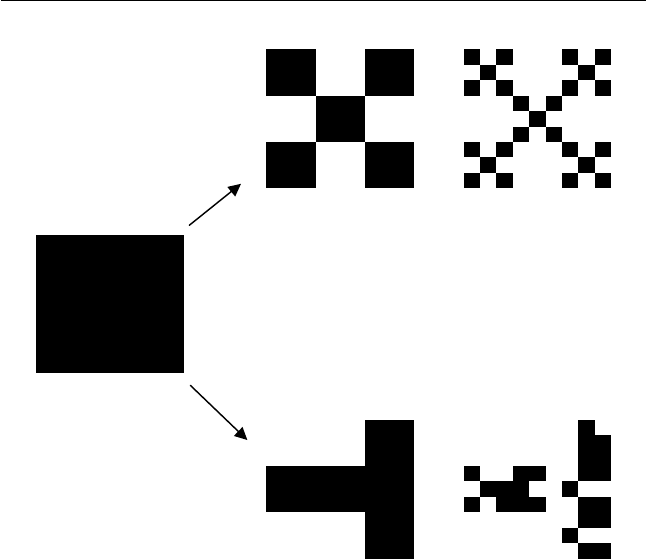
If the geometric pattern used in fractal design is deterministic, the

resulting object is named a deterministic fractal. Consider an example

in path (a) of Figure 6.1 where a square is repeatedly divided into nine

small squares and four of them that have even numbers are deleted

(the squares are numerated along rows). If four squares are deleted at

random, one obtains a random fractal (one of such fractals is depicted

in path (b) of Figure 6.1). While the deterministic and stochastic

fractals in Figure 6.1 look quite different, they have the same fractal

dimension. Let us outline the physical sense of this notion.

Consider a jagged line, such as a coastline. It is embedded into a

plane. Thus, its dimension is lower than two. Yet, the more zigzagged

the line is, the greater part of plane it covers. One may then expect

that the dimension of a coastline is higher than one and it depends on

a measure of jaggedness. Another widely used example is a crumpled

paper ball. It is embedded in three-dimensional space. Yet, the

(a)

(b)

Figure 6.1 Deterministic (a) and stochastic (b) fractals with the same

fractal dimension D ¼ ln(5)/ln(3) .

60 Fractals

volume of a paper ball depends on the sizes of its creases. Therefore,

its dimension is expected to be in the range of two to three. Thus, we

come to the notion of the fractal (non-integer) dimension for objects

that cannot be accurately described within the framework of Eucli-

dian geometry.

There are several technical definitions for the fractal dimension [2].

The most popular one is the box-counting dimension. It implies map-

ping the grid boxes of size h (e.g., squares and cubes for the two-

dimensional and the three-dimensional spaces, respectively) onto the

object of interest. The number of boxes that fill the object is

N(h)  h

D

. The fractal dimension D is then the limit

D ¼ lim

h!0

[ ln N(h)= ln (1=h)] (6:1:1)

The box-counting dimension has another equivalent definition with

the fixed unit size of the grid box and varying object size L

D ¼ lim

L!1

[ ln N(L)= ln (L)] (6:1:2)

The fractal dimension for both deterministic and stochastic fractals in

Figure 6.1 equals D ¼ ln (5)= ln (3)  1:465. Random fractals exhibit

self-similarity only in a statistical sense. Therefore, the scale invari-

ance is a more appropriate concept for random fractals than self-

similarity.

The iterated function systems are commonly used for generating

fractals. The two-dimensional iterated function algorithm for N fixed

points can be presented as

X(k þ 1) ¼ rX(k) þ (1  r)X

F

(i)

Y(k þ 1) ¼ rY(k) þ (1  r)Y

F

(i) (6:1:3)

In (6.1.3), r is the scaling parameter; X

F

(i) and Y

F

(i) are the coordin-

ates of the fixed point i; i ¼ 1, 2, . . . N. The fixed point i is selected at

every iteration at random. A famous example with N ¼ 3, the Sier-

pinski triangle, is shown in Figure 6.2.

Now, let us turn to the random processes relevant to financial time

series. If a random process X(t) is self-affine, then it satisfies the

scaling rule

X(ct) ¼ c

H

X(t) (6:1:4)

Fractals 61