Random Processes: Filtering, Estimation, and Detection

10 Detection Theory: Continuous Observation

 

10.1 CONTINUOUS OBSERVATIONS

The methods presented in the previous sections used a vector of observations. More often the problems we are to solve measure a continuum rather than a finite set. For example, the observed signal x(t) might be recorded for all values of t in the interval from 0 to T. Approaches to the continuous problem are based on expansion of those signals into a weighted sum of CON (complete orthonormal) basis functions. This changes the noncountable problem to a countable infinite one that can be approached by modifying the techniques previously discussed for the finite-dimensional vector case.

For the binary case the problem can be formulated as follows. The observation for class C₁ and class C₂ is x(t) over the interval [0, T] as below:

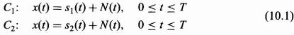
Problems that are mathematically tractable include the special case where N(t) is a realization of a Gaussian white noise random process with known autocorrelation function R_NN(τ) = N₀δ(τ) and power spectral density function ϕ_NN(ω) = N₀ for all ω. The representation above is called an additive white Gaussian noise (AWGN) channel, where x(t) is the received signal, s_i(t) are the signals ...