The R Book

Bootstrap with Regression

An alternative to estimating confidence intervals on the regression parameters from the pooled error variance in the ANOVA table (p. 396) is to use bootstrapping. There are two ways of doing this:

• sample cases with replacement, so that some points are left off the graph while others appear more than once in the dataframe;
• calculate the residuals from the fitted regression model, and randomize which fitted y values get which residuals.

In both cases, the randomization is carried out many times, the model fitted and the parameters estimated. The confidence interval is obtained from the quantiles of the distribution of parameter values (see p. 284).

The following dataframe contains a response variable (profit from the cultivation of a crop of carrots for a supermarket) and a single explanatory variable (the cost of inputs, including fertilizers, pesticides, energy and labour):

regdat<-read.table("c:\\temp\\regdat.txt",header=T)
attach(regdat)
names(regdat)

[1] "explanatory" "response"

plot(explanatory,response)

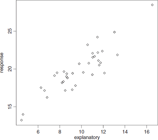
The response is a reasonably linear function of the explanatory variable, but the variance in response is quite large. For instance, when the explanatory variable is about 12, the response variable ranges between less than 20 and more than 24.

model<-lm(response~explanatory)
model

Coefficients:
(Intercept)   explanatory
      9.630         1.051

Theory suggests ...