The R Book

Estimating LD50 and LD90 from bioassay data

The data consist of numbers dead and initial batch size for five doses of pesticide application, and we wish to know what dose kills 50% of the individuals (or 90% or 95%, as required). The tricky statistical issue is that one is using a value of y (50% dead) to predict a value of x (the relevant dose) and to work out a standard error on the x axis.

data<-read.table("c:\\temp\\bioassay.txt",header=T)
attach(data)
names(data)

[1]  "dose" "dead" "batch"

The logistic regression is carried out in the usual way:

y<-cbind(dead,batch-dead)
model<-glm(y~log(dose),binomial)

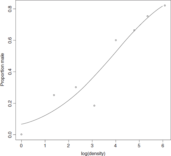
Then the function dose.p from the MASS library is run with the model object, specifying the proportion killed (p = 0.5 is the default for LD50):

library(MASS)
dose.p(model,p=c(0.5,0.9,0.95))
              Dose           SE
p = 0.50: 2.306981    0.07772065
p = 0.90: 3.425506    0.12362080
p = 0.95: 3.805885    0.15150043

Here the logs of LD50, LD90 and LD95 are printed, along with their standard errors.

Proportion data with categorical explanatory variables

This next example concerns the germination of seeds of two genotypes of the parasitic plant Orobanche and two extracts from host plants (bean and cucumber) that were used to stimulate germination. It is a two-way factorial analysis of deviance.

germination<-read.table("c:\\temp\\germination.txt",header=T)
attach(germination)
names(germination) [1] "count" ...