The R Book

Nicholson's Blowflies

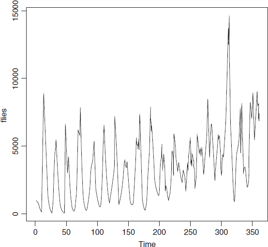
The Australian ecologist, A.J. Nicholson, reared blowfly larvae on pieces of liver in laboratory cultures that his technicians kept running continuously for almost 7 years (361 weeks, to be exact). The time series for numbers of adult flies looks like this:

blowfly<-read.table("c:\\temp\\blowfly.txt",header=T)
attach(blowfly)
names(blowfly)

[1] "flies"

First, make the flies variable into a time series object:

flies<-ts(flies)

and plot it:

plot(flies)

This classic time series has two clear features:

• For the first 200 weeks the system exhibits beautifully regular cycles.
• After week 200 things change (perhaps a genetic mutation had arisen); the cycles become much less clear-cut, and the population begins a pronounced upward trend.

There are two important ideas to understand in time series analysis: autocorrelation and partial autocorrelation. The first describes how this week's population is related to last week's population. This is the autocorrelation at lag 1. The second describes the relationship between this week's population and the population at lag t once we have controlled for the correlations between all of the successive weeks between this week and week t. This should become clear if we draw the scatterplots from which the first four autocorrelation terms are calculated (lag 1 to lag 4).

There is a snag, however. The vector of flies at lag 1 ...