The R Book, 2nd Edition

Chapter 13

Generalized Linear Models

We can use generalized linear models (GLMs) – pronounced ‘glims’ – when the variance is not constant, and/or when the errors are not normally distributed. Certain kinds of response variables invariably suffer from these two important contraventions of the standard assumptions, and GLMs are excellent at dealing with them. Specifically, we might consider using GLMs when the response variable is:

• count data expressed as proportions (e.g. logistic regressions);
• count data that are not proportions (e.g. log-linear models of counts);
• binary response variables (e.g. dead or alive);
• data on time to death where the variance increases faster than linearly with the mean (e.g. time data with gamma errors).

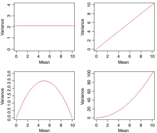
The central assumption that we have made up to this point is that variance was constant (top left-hand graph). In count data, however, where the response variable is an integer and there are often lots of zeros in the dataframe, the variance may increase linearly with the mean (top tight). With proportion data, where we have a count of the number of failures of an event as well as the number of successes, the variance will be an inverted U-shaped function of the mean (bottom left). Where the response variable follows a gamma distribution (as in time-to-death data) the variance increases faster than linearly with the mean (bottom right). Many of the ...