The Value of Debt: How to Manage Both Sides of a Balance Sheet to Maximize Wealth

Appendix D

Some Examples of Ideal Debt Ratios*

This appendix will help to frame the concept of optimal by sketching out what a number of different optimal debt ratios look like in practice. Since some of these materials are a bit more advanced, we will use the same format we used at the end of Chapter 5, which is to lay out two balance sheets in a side-by-side comparison. We will start out with a review of a case study from Chapter 5 and then continue on to increasingly more advanced scenarios and concepts.

Scenario 1: “I’m an Accumulator—No Debt for Me!”

(This is the same scenario for Jane earlier reviewed in Chapter 5.)

In the optimal scenario, on the right of Table D.1, Jane

Table D.1 Scenario 1: “I'm an Accumulator—No Debt for Me!”

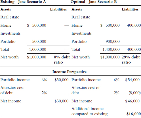
• Generates $16,000 more per year in income, which is equivalent to increasing her rate of return by 53.3 percent.
• Gets a significant tax deduction (the benefit of this is accounted for in her after-tax cost of debt).
• Is eligible for an ABLF that is 80 percent higher and likely priced at a lower rate.
• Is not subject to a forced margin call because her debt is structured against her home.
• Can pay off her debt anytime she doesn’t like this strategy.

If Jane reinvests the additional $16,000 at the same 6 percent for five years, she will generate a total of approximately $90,000 in additional value versus the no-debt scenario on the left.

Looking forward: ...