
 Filter (source: Pixabay)
 Given all of the higher level tools that you can use with TensorFlow, such as tf.contrib.learn and Keras, one can very easily build a convolutional neural network with a very small amount of code. But often with these higher level applications, you cannot access the little inbetween bits of the code, and some of the understanding of what’s happening under the surface is lost.
In this tutorial, I’ll walk you through how to build a convolutional neural network from scratch, using just the low-level TensorFlow and visualizing our graph and network performance using TensorBoard. If you don’t understand some of the basics of a fully connected neural network, I highly recommend you first check out Not another MNIST tutorial with TensorFlow. Throughout this article, I will also break down each step of the convolutional neural network to its absolute basics so you can fully understand what is happening in each step of the graph. By building this model from scratch, you can easily visualize different aspects of the graph so that you can see each layer of convolutions and use them to make your own inferences. I will only highlight major aspects of the code, so if you would like to follow this code step-by-step, you can checkout the corresponding Jupyter Notebook on GitHub.
Gathering a data set
Getting started, I had to decide which image data set to use. I decided to use the University of Oxford, Visual Geometry Group’s pet data set. I chose this data set for a few reasons: it is very simple and well-labeled, it has a decent amount of training data, and it also has bounding boxes—to utilize if I want to train a detection model down the road. Another data set I thought would be excellent for a building a first model was the Simpsons data set found on Kaggle, which has a great amount of simple data on which to train.
Choosing a model
Next, I had to decide on the model of my convolutional neural network. Some very popular models are GoogLeNet or VGG16, which both have multiple convolutions designed to detect images from the 1000 class data set imagenet. I decided on a much simpler four convolutional network:
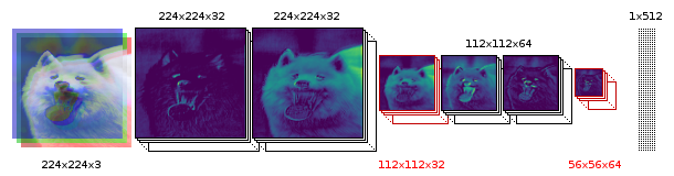
To break down this model, it starts with a 224x224x3 image, which is is convolved to 32 feature maps, based from the previous three channels. We than convolve this group of 32 feature maps together into another 32 features. This is then pooled into a 112x112x32 image, which we convolve into 64 feature maps twice followed, with a final pooling of 56x56x64. Each unit of this final pooled layer is then fully connected to 512 neurons, and then finally put through a softmax layer based upon the number of classes.
Processing and building a data set
First, let’s get started with loading our dependencies, which includes a group of helper functions I made called imFunctions for processing the image data.
importimFunctionsasimfimporttensorflowastfimportscipy.ndimagefromscipy.miscimportimsaveimportmatplotlib.pyplotaspltimportnumpyasnp
We can then download and extract the images using imFunctions.
imf.downloadImages('annotations.tar.gz',19173078)imf.downloadImages('images.tar.gz',791918971)imf.maybeExtract('annotations.tar.gz')imf.maybeExtract('images.tar.gz')
We can then sort the images into separate folders, including training and test folders. The number in the sortImages function represents the percentage of test data you would like to separate from the training data.
imf.sortImages(0.15)
We can then build our data set into a numpy array with a corresponding one hot vector to represent our class. This will also subtract the image mean from all of the training and test imagesa standard practice when building a convnet. The function will ask you what classes you would like to include—due to my limited amount of GPU ram (3GB), I choose a very small data set that tries to differentiate two breeds of dogs: a Shiba Inu from a Samoyed.
train_x,train_y,test_x,test_y,classes,classLabels=imf.buildDataset()
How convolutions and pooling work
Now that we have a data set to work with, let’s step back a bit and look at the absolute basics of how convolutions work. Before jumping into a color convolutional filter, let’s look at a grayscale one to make sure everything is clear. Let’s make a 7×7 filter that applies four different feature maps. TensorFlow’s conv2d function is fairly simple and takes in four variables: input, filter, strides, and padding. On the TensorFlow site, they describe the conv2d function as follows:
Computes a 2-D convolution given 4-D input and filter tensors.
Given an input tensor of shape [batch, in_height, in_width, in_channels] and a filter / kernel tensor of shape [filter_height, filter_width, in_channels, out_channels].
Since we are working with grayscale, the in_channels will be 1, and since we are applying four filters our out_channels will be 4. Let’s apply the following four filters/kernels to just one of our images, or a batch of 1:
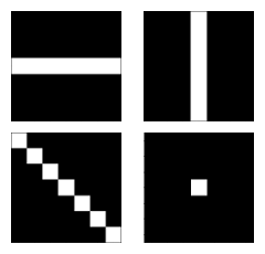
And let’s see how this filter affected our grayscaled image input.
gray=np.mean(image,-1)X=tf.placeholder(tf.float32,shape=(None,224,224,1))conv=tf.nn.conv2d(X,filters,[1,1,1,1],padding="SAME")test=tf.Session()test.run(tf.global_variables_initializer())filteredImage=test.run(conv,feed_dict={X:gray.reshape(1,224,224,1)})tf.reset_default_graph()
This will return a 4d tensor of (1, 224, 224, 4), which we can use to visualize the four filters:
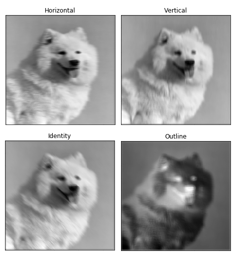
It’s clear to see that convolutions of filter kernels are very powerful. To break it down, our 7×7 kernel is striding in steps of one over 49 of the image’s pixels at a time, the value of each pixel is then multiplied by each kernel value, and then all of the 49 values are added together to make one pixel. If the idea of image filter kernels is still not making sense, I highly recommend this website—they do an excellent job of visualizing kernels.
Now, in essence, most convolutional neural networks consist of just convolutions and poolings. Most commonly, a 3×3 kernel filter is used for convolutions. Particularly, max poolings with a stride of 2×2 and kernel size of 2×2 are just an aggressive way to essentially reduce an image’s size based upon its maximum pixel values within a kernel. Here is a basic example of a 2×2 kernel with a stride of 2 in both dimensions.
Now, for both conv2d and max pooling, there are two options to choose from for padding: “VALID,” which will shrink an input and “SAME,” which will maintain the inputs size by adding zeros around the edges of the input. Here is an example of a max pool with a 3×3 kernel, with a stride of 1×1 to compare the padding options:
Building the convnet
Now that we’ve got the basics covered, let’s start building our convolutional neural network model. We can start with our placeholders. X will be our input placeholder, which we will feed our images into, and Y_ will be the true classes of a set of images.
X=tf.placeholder(tf.float32,shape=(None,224,224,3))Y_=tf.placeholder(tf.float32,[None,classes])keepRate1=tf.placeholder(tf.float32)keepRate2=tf.placeholder(tf.float32)
We will create all parts for each process under one scope. Scope’s are extremely useful for visualizing the graph in TensorBoard down the road because they will group everything into one expandable object. We create our first set of filters with a kernel size of 3×3, which takes in three channels and outputs 32 filters. This means that for every one of the 32 filters, there will be 3×3 kernel weights for the R, G, and B channels. It’s very important that the weight values for our filter are initialized using truncated normal so we have multiple random filters that TensorFlow will adapt to fit our model.
# CONVOLUTION 1 - 1withtf.name_scope('conv1_1'):filter1_1=tf.Variable(tf.truncated_normal([3,3,3,32],dtype=tf.float32,stddev=1e-1),name='weights1_1')stride=[1,1,1,1]conv=tf.nn.conv2d(X,filter1_1,stride,padding='SAME')biases=tf.Variable(tf.constant(0.0,shape=[32],dtype=tf.float32),trainable=True,name='biases1_1')out=tf.nn.bias_add(conv,biases)conv1_1=tf.nn.relu(out)
At the end of our first convolution, conv1_1, we finish off by applying relu, which acts as a threshold by assigning every negative number to zero. We then convolve those 32 features together into another 32 features. You can see conv2d assigns the input to be the output of the first convolutional layer.
# CONVOLUTION 1 - 2withtf.name_scope('conv1_2'):filter1_2=tf.Variable(tf.truncated_normal([3,3,32,32],dtype=tf.float32,stddev=1e-1),name='weights1_2')conv=tf.nn.conv2d(conv1_1,filter1_2,[1,1,1,1],padding='SAME')biases=tf.Variable(tf.constant(0.0,shape=[32],dtype=tf.float32),trainable=True,name='biases1_2')out=tf.nn.bias_add(conv,biases)conv1_2=tf.nn.relu(out)
We then pool to shrink the image in half.
# POOL 1withtf.name_scope('pool1'):pool1_1=tf.nn.max_pool(conv1_2,ksize=[1,2,2,1],strides=[1,2,2,1],padding='SAME',name='pool1_1')pool1_1_drop=tf.nn.dropout(pool1_1,keepRate1)
This last part involves using dropout on the pool layer (we will go into more detail on that later). We then follow with two more convolutions, with 64 features and another pool. Notice that the first convolution has to convert the previous 32 feature channels into 64.
# CONVOLUTION 2 - 1withtf.name_scope('conv2_1'):filter2_1=tf.Variable(tf.truncated_normal([3,3,32,64],dtype=tf.float32,stddev=1e-1),name='weights2_1')conv=tf.nn.conv2d(pool1_1_drop,filter2_1,[1,1,1,1],padding='SAME')biases=tf.Variable(tf.constant(0.0,shape=[64],dtype=tf.float32),trainable=True,name='biases2_1')out=tf.nn.bias_add(conv,biases)conv2_1=tf.nn.relu(out)# CONVOLUTION 2 - 2withtf.name_scope('conv2_2'):filter2_2=tf.Variable(tf.truncated_normal([3,3,64,64],dtype=tf.float32,stddev=1e-1),name='weights2_2')conv=tf.nn.conv2d(conv2_1,filter2_2,[1,1,1,1],padding='SAME')biases=tf.Variable(tf.constant(0.0,shape=[64],dtype=tf.float32),trainable=True,name='biases2_2')out=tf.nn.bias_add(conv,biases)conv2_2=tf.nn.relu(out)# POOL 2withtf.name_scope('pool2'):pool2_1=tf.nn.max_pool(conv2_2,ksize=[1,2,2,1],strides=[1,2,2,1],padding='SAME',name='pool2_1')pool2_1_drop=tf.nn.dropout(pool2_1,keepRate1)
Next, we create a 512 neuron, fully connected layer, which will have a weight connection for each pixel of our 56x56x64 pool2_1 layer. That’s more than 100 million different weight values! In order to calculate our fully connected network, we have to flatten the input into one dimension, and then we can multiply it by our weights and add our bias.
#FULLY CONNECTED 1withtf.name_scope('fc1')asscope:shape=int(np.prod(pool2_1_drop.get_shape()[1:]))fc1w=tf.Variable(tf.truncated_normal([shape,512],dtype=tf.float32,stddev=1e-1),name='weights3_1')fc1b=tf.Variable(tf.constant(1.0,shape=[512],dtype=tf.float32),trainable=True,name='biases3_1')pool2_flat=tf.reshape(pool2_1_drop,[-1,shape])out=tf.nn.bias_add(tf.matmul(pool2_flat,fc1w),fc1b)fc1=tf.nn.relu(out)fc1_drop=tf.nn.dropout(fc1,keepRate2)
Last, we have our softmax with its associated weights and bias, and finally our output Y.
#FULLY CONNECTED 3 & SOFTMAX OUTPUTwithtf.name_scope('softmax')asscope:fc2w=tf.Variable(tf.truncated_normal([512,classes],dtype=tf.float32,stddev=1e-1),name='weights3_2')fc2b=tf.Variable(tf.constant(1.0,shape=[classes],dtype=tf.float32),trainable=True,name='biases3_2')Ylogits=tf.nn.bias_add(tf.matmul(fc1_drop,fc2w),fc2b)Y=tf.nn.softmax(Ylogits)
Create loss & optimizer
Now, we can start developing the training aspect of our model. First, we have to decide the batch size; I couldn’t use more than 10 without running out of GPU memory. Then we have to decide the number of epochs, which is the number of times the algorithm will cycle through all the training data in batches, and lastly our learning rate alpha.
numEpochs=400batchSize=10alpha=1e-5
We then create some scopes for our cross entropy, accuracy checker, and back propagation optimizer.
withtf.name_scope('cross_entropy'):cross_entropy=tf.nn.softmax_cross_entropy_with_logits(logits=Ylogits,labels=Y_)loss=tf.reduce_mean(cross_entropy)withtf.name_scope('accuracy'):correct_prediction=tf.equal(tf.argmax(Y,1),tf.argmax(Y_,1))accuracy=tf.reduce_mean(tf.cast(correct_prediction,tf.float32))withtf.name_scope('train'):train_step=tf.train.AdamOptimizer(learning_rate=alpha).minimize(loss)
We can then create our session and initialize all our variables.
sess=tf.Session()init=tf.global_variables_initializer()sess.run(init)
Create summaries for TensorBoard
Now, we also will want to utilize TensorBoard so we can visualize how well our classifier is doing. We will create two plots: one for our training set and one for our test set. We can visualize our graph network by using the add_graph function. We will measure our total loss and accuracy using summary scalar, and merge our summaries together so we only have to call write_op to log our scalars.
writer_1=tf.summary.FileWriter("/tmp/cnn/train")writer_2=tf.summary.FileWriter("/tmp/cnn/test")writer_1.add_graph(sess.graph)tf.summary.scalar('Loss',loss)tf.summary.scalar('Accuracy',accuracy)tf.summary.histogram("weights1_1",filter1_1)write_op=tf.summary.merge_all()
Train the model
We then can set up our code for evaluation and training. We don’t want to use our summary writer for our loss and accuracy for every time step, as this would greatly slow down the classifier. So instead, we log every five steps.
steps=int(train_x.shape[0]/batchSize)foriinrange(numEpochs):accHist=[]accHist2=[]train_x,train_y=imf.shuffle(train_x,train_y)foriiinrange(steps):#Calculate our current stepstep=i*steps+ii#Feed forward batch of train images into graph and log accuracyacc=sess.run([accuracy],feed_dict={X:train_x[(ii*batchSize):((ii+1)*batchSize),:,:,:],Y_:train_y[(ii*batchSize):((ii+1)*batchSize)],keepRate1:1,keepRate2:1})accHist.append(acc)ifstep%5==0:# Get Train Summary for one batch and add summary to TensorBoardsummary=sess.run(write_op,feed_dict={X:train_x[(ii*batchSize):((ii+1)*batchSize),:,:,:],Y_:train_y[(ii*batchSize):((ii+1)*batchSize)],keepRate1:1,keepRate2:1})writer_1.add_summary(summary,step)writer_1.flush()# Get Test Summary on random 10 test images and add summary to TensorBoardtest_x,test_y=imf.shuffle(test_x,test_y)summary=sess.run(write_op,feed_dict={X:test_x[0:10,:,:,:],Y_:test_y[0:10],keepRate1:1,keepRate2:1})writer_2.add_summary(summary,step)writer_2.flush()#Back propigate using adam optimizer to update weights and biases.sess.run(train_step,feed_dict={X:train_x[(ii*batchSize):((ii+1)*batchSize),:,:,:],Y_:train_y[(ii*batchSize):((ii+1)*batchSize)],keepRate1:0.2,keepRate2:0.5})('Epoch number {} Training Accuracy: {}'.format(i+1,np.mean(accHist)))#Feed forward all test images into graph and log accuracyforiiiinrange(int(test_x.shape[0]/batchSize)):acc=sess.run(accuracy,feed_dict={X:test_x[(iii*batchSize):((iii+1)*batchSize),:,:,:],Y_:test_y[(iii*batchSize):((iii+1)*batchSize)],keepRate1:1,keepRate2:1})accHist2.append(acc)("Test Set Accuracy: {}".format(np.mean(accHist2)))
Visualize graph
While this is training, let’s check out the TensorBoard results by activating TensorBoard in the terminal.
tensorboard--logdir="/tmp/cnn/"
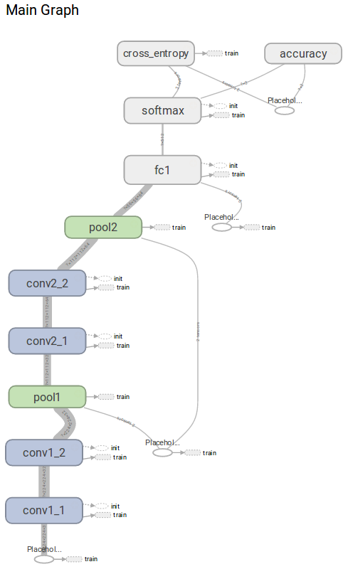
We can then direct our web browser to the default TensorBoard address http://0.0.0.0/6006. Let’s first look at our graph model.
As you can see, by using scopes we are able to visualize a nice clean version of our graph.
Measure performance
Let’s check out the scalar history for our accuracy and loss.
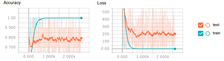
You may be able to tell that we have a huge problem. For our training data, the classifier is getting 100% accuracy and 0 loss, but our test data is only achieving 80% at best and still getting a lot of loss. This is your obvious sign of overfitting—some classic symptoms include not enough training data, or having too many neurons.
We could create more training data by resizing, scaling, and rotating our training data, but a much easier approach is to add dropout to the output of our pooling and fully connected layers. This will make every training step completely cut, or drop out, a percentage of neurons randomly, in a layer. This will force our classifier to only train small sets of neurons at a time, rather than the whole set. This allows neurons to specialize in specific tasks, rather than all neurons generalizing together. Dropping out 80% of our convolutional layers and 50% of our fully connected layers gives some amazing results.
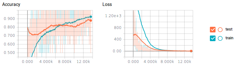
Just by dropping off neurons, we were able to achieve just under 90% on our test data—that is almost a 10% increase in performance! One drawback is that the classifier took about 6x longer to train.
Visualize evolving filters
For extra fun, for every 50 training steps, I passed an image through a filter and made a gif of the filters’ weights evolving. It resulted in some pretty cool effects and some really good insight on how the convolutional network was working. Here are two filters from conv1_2:
You can see the initial weight initialization shows a lot of the image, but as the weights updated over time, they became more focused on detecting certain edges. To my surprise, I discovered that the very first convolutional kernel, filter1_1, hardly changed at all. It seemed that the beginning weight initializations did good enough on their own. Going further down the network, here is conv2_2—you can see it beginning to detect more abstract generalized features.
All in all, I was extremely impressed that I was able to train a model with almost 90% accuracy using less than 400 training images. I’m sure with more training data, and more tweaking of the hyperparameters, I could have achieved even better results.
This concludes how to create a convolutional neural network from scratch using TensorFlow, and how to gain inferences from TensorBoard and by visualizing our filters. It’s important to remember that a much easier method when making a classifier with little data is to take a model and weights that have already been trained on a huge data set with multiple GPUs, such as GoogLeNet or VGG16, and cut off the very last layer and replace them with their own classes. Then, all the classifier has to do is learn the weights for the very last layer and use the pre-existing trained filter weights. So, I hope you got something out of this post and go forth, have fun, experiment, learn, and visualize!
This post is a collaboration between O’Reilly and TensorFlow. See our statement of editorial independence.