Half the transmit power I pump into my antenna is wasted. The trouble is that I don’t know which half.
In its most basic conception, MIMO is technology that provides a multi-lane highway for 802.11n transmissions. When a transmitter can send multiple streams across a link, throughput improves. This description of MIMO is fairly passive, and does not provide a full picture of everything that a MIMO system can do. With an antenna array, it is possible to create far more sophisticated transmissions than just sending multiple streams. With advanced radio chips, it is possible to send transmissions from the MIMO antenna array in a particular direction in a process called beamforming. Individual receiving antennas within MIMO arrays can also cross-check each other to improve signal processing at the receiver. Both applications can increase the signal to noise ratio, which improves speed. In addition to developing the underlying technology for antenna arrays, 802.11n includes protocol features that can improve the signal processing gain. MIMO can also be used to spread a single spatial stream across multiple transmitters for extra signal-processing gain at the receiver, and hence, longer range in a process called Space-Time Block Coding (STBC). 802.11n also provides another option to increase signal-processing gain, the Low-Density Parity Check (LDPC) code. As discussed in Relationship Between Spatial Streams and Radio Chains, many products also implement some form of ratio combining to increase signal gain, though ratio combining is not a protocol feature.
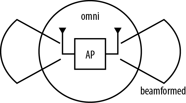
Prior to 802.11n, most access points were equipped by default with omnidirectional antennas. “Omnis” radiate equally in all directions, and their coverage is often depicted as a circle with the AP at the center. One of the costs of of an omni is that the signal destined to a receiver is sprayed out evenly in all directions, even though the receiver is only in one of those directions. The best way I have found to explain it is to recall John Wanamaker’s famous statement that half of all advertising spending is wasted, but the problem is that nobody knows which half goes to waste. Beamforming is 802.11’s answer to this conundrum. It enables an antenna array to focus the energy in the direction of a client device. By using the same power but focusing it towards the receiver, it is possible to increase the signal to noise ratio at the receiver. Higher signal to noise ratio enables use of more aggressive coding, and therefore, higher speed. Figure 4-1 shows the basic idea of beamforming. A transmitter, also called the beamformer, “focuses” or “steers” the energy so that the transmission tends to go more in one direction, towards the receiver, also called a beamformee. (The terms beamformer and beamformee are useful in the context of explicit channel measurement protocols that require frame exchanges.) The figure illustrates one of the classic beamforming trade-offs. To form a beam in one direction, the result is often a figure-8 coverage pattern, as shown in the figure.
In essence, beamforming is an electrically steerable antenna. When transmitting to a given receiver, the antenna is “pointed” in the direction of the receiver, but the direction that the beam is focused can be controlled by subtly altering the phase shifts into the antenna system rather than mechanically moving the antenna. Phase shifts in the transmission sent by each antenna are used to focus energy along lines of constructive interference between the antenna elements.[20]
Naturally, phase shifting the transmissions to individual radio chains requires fairly advanced signal processing within the 802.11 chip. When the transmission is biased towards transmission in one direction, it tends to have a relatively low sensitivity in the opposite direction. For example, in Figure 4-1, the beam is being focused at the receiver on the right. Interference sources from other directions will tend to be rejected by the antenna because the antenna system is pushing the gain towards the right.
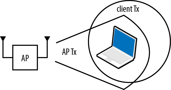
By concentrating radio energy in a particular direction, the “downstream” link from AP to client gets additional power. With more power, a stronger signal is better able to cut through interference. A gain of just 1-2 dB can be the difference between data rates in an 802.11 device.[21] The disadvantage of beamforming is that its benefits are concentrated at the receiver. Figure 4-2 illustrates the point by showing a typical network with an AP and a laptop attached to it. When the AP transmits to the laptop, it is able to transmit a concentrated beam, potentially with a gain over an omindirectional antenna of 3-5 dB. However, when the laptop sends the 802.11 ACK (or a TCP segment containing a TCP-layer acknowledgment), the AP cannot set up the antenna with sensitivity “pointing at” the client because it may be serving multiple attached client devices. 802.11 does not exercise tight control over transmission timing, so beamforming access points generally receive without any steering and are restricted to using antenna arrays as omnidirectional receivers. As a result, beamforming generally leads to asymmetric links, with the potential for hidden node interference. To eliminate link asymmetry or reduce its negative effects, focus on the receive sensitivity of the AP to offset the lower receive antenna gain.
Warning
Asymmetric links are not compatible with all applications. If the transmissions mainly flow downstream from an AP to receivers, it can increase speed. Balanced links that expect upstream data (such as voice or videoconferencing) may not see much gain from beamforming, especially if RTS/CTS exchanges are required to avoid hidden nodes.
Beamforming refers to one of several related technologies that can be used to increase SNR at the receiver. This book uses the term beamforming to refer only to technologies that work by actively steering transmissions from an antenna array by using multiple antenna array elements. If your transmitter isn’t using multiple components in an array to steer the beam, it’s not beamforming. For example, an array of static directional antennas doesn’t do beamforming. It may increase range by using high-gain directional antennas, but it is using the directional antennas in a static way. To be a true beamforming device, either the radio chip or the antenna must be doing something to change the transmissions out of an antenna array, and do so on a frame-by-frame basis.
Whether implemented on the radio chip or in the antenna array, beamforming works by taking the radio signals to be transmitted and applying a mathematical transformation to them that changes the way they are transmitted. Mathematically, the transformation is typically represented as a matrix that takes an incoming signal pre-beamforming and maps it to a number of outputs.[22] With on-chip beamforming, the matrix has dimensions of the number of space-time streams that are inputs and the number of transmit chains. In a 3-stream system with 3 outputs, the matrix will be a square that maps some combination of the inputs to each of the outputs. When beamforming is implemented in the antenna array, the size of the matrix is also the number of inputs and outputs. An antenna array may still take the 3-stream transmission as input, but instead of mapping on to three transmit chains, the antenna may map those three inputs on to ten or more output elements.
The matrix that describes the transformation from space-time streams to transmitted energy is called the steering matrix. In the block diagram of an 802.11n interface in Figure 3-7, the spatial mapper uses the steering matrix to alter the transmitted data to have longer reach. A similar process would be carried out within software running on the antenna system in an antenna-based beamforming system.
Broadly speaking, beamforming comes in two major flavors, and both are compared in Table 4-1. Explicit beamforming is easy to understand. Before transmitting, a device actively measures the channel, and uses the measurement to compute the steering matrix directly. Active channel measurement is accomplished by transmitting a sounding frame to the beamformee, which replies with a frame that indicates how the sounding frame was received. By comparing the known contents of the sounding frame to a representation of its contents at the receiver, the beamformer can compute the steering matrix. The downside to explicit beamforming is that it requires active support on both ends of the radio link. To receive beamformed transmissions, a device must be able to send channel measurements back to the beamformer. Only 802.11n has defined the channel measurement sequences, which means that older 802.11a/g devices will be unable to receive explicit beamformed frames.
Almost all 802.11n access points that support beamforming do so based on implicit beamforming. As the name implies, implicit beamforming devices do not use any frame exchanges that are dedicated to beamforming. Instead, devices estimate the beamforming matrix from received frames, or by inference from frames that are lost. Well-known frames such as ACKs or the data transmitted on pilot channels can be used to estimate the steering matrix. Implicit beamforming is based on less comprehensive measurements, and therefore, does not provide quite as high a level of performance. On the other hand, the implicit variety may be implemented by only one side of a link and may be used when that link supports a pre-11n PHY. For these reasons, implicit beamforming is significantly more common, and serves as a bridge between traditional omnidirectional transmission and the future of standards-based beamforming in 802.11 radio chips.
Table 4-1. Beamforming technology comparison
| Attribute | Implicit | Explicit |
|---|---|---|
| 802.11 PHY support | 802.11a, b, g, and n | 802.11n only |
| Client requirement | None | Send channel measurements to AP |
| Link adaptation | Open loop | Closed loop |
| Feedback source | Client uplink frames | Client channel measurements |
| Performance gain | Moderate gain, generally increasing with the number of antenna elements | Higher gain |
| Implementation location | Software/firmware built into antenna system or layered on top of radio chip | Special features within 802.11n radio interface |
| Number of implementations | Common | Rare |
Space-Time Block Coding (STBC) can be used when the number of radio chains exceeds the number of spatial streams. In effect, STBC transmits the same data stream twice across two spatial streams so that a receiver that misses a data block from one spatial stream has a second shot at decoding the data on the second spatial stream. In effect, STBC takes the gains from MIMO and uses them nearly exclusively for increased range. A single encoding stream must take two radio chains for transmission, which means that a 2×2 MIMO device transmitting with STBC is effectively operating as a single-stream device. 802.11 interfaces include a step-down algorithm that selects slower and more reliable transmission rates; STBC can be used when the data channel is too poor to support one full stream per radio. In such environments, STBC is worth the 50% penalty on transmitted speed. When an STBC-enabled AP is serving mainly single-stream devices at long ranges, STBC is definitely worth considering.
Until 802.11n, all OFDM-based PHYs used a convolutional code as the forward-error correcting (FEC) code. Conceptually, a convolutional code works by “smearing out” errors over time so that a single bit error can be corrected if enough neighboring bits are good. The low-density parity check (LDPC) code that is defined as an option in 802.11n works in a similar manner, but it also offers a coding gain when compared to convolutional codes. Depending on the channel model, simulations show that LDPC increases signal-to-noise ratio between 1.5 and 3 dB.[23]
The LDPC operates on code words that are 648 bits, 1296 bits, or 1944 bits long. When a frame is sent to the 802.11n interface for transmission, it is first divided into blocks based on the length of the code word (Table 4-2). As with the convolutional code, the coding rate defines the number of added bits used to detect and correct errors; no change is required to the tables in Comparison 2: 20 MHz versus 40 MHz channels.
Table 4-2. LDPC block size and rates
| Code rate | Data bits per code word |
|---|---|
| R=1/2 | 324, 648, or 972 |
| R=2/3 | 432, 864, or 1296 |
| R=3/4 | 486, 972, or 1458 |
| R=5/6 | 540, 1080, or 1620 |
Use of LDPC must be negotiated as part of the 802.11 association process. An 802.11n device only transmits LDPC-encoded frames to peers that have indicated support for LDPC in either Beacon frames or Association Request frames.
[20] In most beamforming systems, the antenna array is still composed of omnidirectional antennas. Complex phased-array antenna systems with many elements can be used as well, but such antennas have significantly higher complexity, and hence, cost. Expensive antenna arrays make a great deal of sense in mobile telephony; when used in Wi-Fi APs, the antenna array tends to lead to compromises in other areas of the system design.
[21] Although it doesn’t really sound like it, 1 dB is a huge amount in the radio world. Don’t believe me? Go ask your boss for a “1 dB raise.”
[22] Matrix operations are used because the effects of multipath interference may be different for each spatial stream. Beamforming is used independently for each stream because each stream may have different frequency-specific fading effects.
[23] One of the early presentations on LDPC’s coding gain is IEEE document 11-04/0071.
Get 802.11n: A Survival Guide now with the O’Reilly learning platform.
O’Reilly members experience books, live events, courses curated by job role, and more from O’Reilly and nearly 200 top publishers.

