Anonymizing Health Data

Chapter 4. Longitudinal Discharge Abstract Data: State Inpatient Databases

After patients are discharged from a hospital—in some cases months after—their medical information is organized and cleaned up to accurately reflect their stay in the hospital. The resulting document is known as a discharge abstract. A State Inpatient Database (SID) is a collection of all Discharge Abstract Data (DAD) for a state, and it’s a powerful tool for research and analysis to inform public policy.^[48]

The SID databases for many states are made available for research and other purposes. But there have been concerns raised about how well they’ve been de-identified when shared,^[49] and some have been successfully attacked.^[50] We’ll provide some analysis to inform de-identification practices for this kind of data, and we’ll look at methods that can be used to create a public use SID.

Note

In addition to quasi-identifiers, a data set can contain sensitive information such as drugs dispensed or diagnoses. This information could be used to infer things like mental health status or disabilities. We don’t consider that kind of sensitive information in the analysis here, for ease of presentation, but just assume that it exists in the data sets we refer to. Re-identifying patients therefore implies potentially learning about sensitive information that patients might not want others to know about.

While we’ll present de-identification algorithms here in the context of longitudinal data, any multilevel data set can be de-identified using these methods as well. A birth registry with maternal information at the first level could, for example, be combined with information about each baby at the second level, or data about cancer patients at the top level could be combined with data about their family members who’ve had cancer at the second level.

Longitudinal Data

Over a period of time, patients can make multiple hospital or clinic visits, and linking a patient’s records throughout is what makes the data longitudinal. Data sets of this type need to be de-identified differently from cross-sectional data. If you try to de-identify a longitudinal data set using methods developed for cross-sectional data, you’ll either do too little to protect the patients properly, or you’ll do too much and distort the data to the point where it becomes useless.

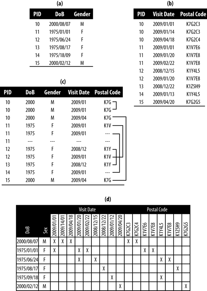
We can understand this principle by looking at the example of longitudinal data in Figure 4-1. There are six patients with basic demographics in panel (a), and their visit information in panel (b). ZIP codes were collected at each visit in case patients moved. The patients with IDs 10 and 11 had three visits each in 2009, whereas patient 12 had only two visits: one in 2008 and one in 2009. The patient ID (PID) is used to identify the visits that belong to a patient—without it we’d lose the longitudinal nature of the data set, and lose the chance to do any analysis benefitting from a survey of multiple visits by a patient. In addition, at least for this data set, we wouldn’t be able to link to patient demographics.

Figure 4-1. Demographics (a) and visits (b), joined and 2-anonymized (c), with a binary view (d) for good measure

Don’t Treat It Like Cross-Sectional Data

k-anonymization techniques using generalization and suppression for de-identifying cross-sectional data won’t work as intended on longitudinal data. To see why, let’s try some techniques from the previous chapter on our example longitudinal data and see the problems that arise:

Suppression in single records

One way to represent the longitudinal data in Figure 4-1 is to join the two tables in panels (a) and (b) and have a single data set of patient visits. Each patient can appear multiple times in the joined data set. Panel (c) in Figure 4-1 shows what this de-identified data set with 2-anonymity would look like. The postal code for patient number 11 was suppressed in her second visit, and all quasi-identifiers for her third visit were suppressed. But k-anonymity treats each record as an independent observation, ignoring the PID entirely. An adversary could see that the first and second visit are in the same month, and guess that the first three digits of the patient’s postal code won’t have changed. The postal code was suppressed to achieve 2-anonymity, but it didn’t actually work as intended.

Homogeneous equivalence classes

The probability of re-identifying a patient is not necessarily as low as intended when applying current k-anonymity algorithms to longitudinal data. Under k-anonymity, the first two records in panel (c) of Figure 4-1 form an equivalence class. But the records belong to the same patient, so the probability of re-identifying the patient is 1 despite having k = 2.

Detailed background knowledge

Let’s say that an adversary wants to re-identify Alice in the data. The adversary has collected some information about her and knows that she’s made at least a couple of visits to the hospital. In our example data, two female patients have made at least two visits to the hospital. But the adversary knows that Alice’s visits were in “2008/11 and 2009/01.” That makes her PID 12. Because k-anonymity treats a data set as cross-sectional, patterns that span multiple records (i.e., longitudinal patterns) are not protected.

Another way to represent such longitudinal data is by creating a variable for each quasi-identifier. This is referred to as binary or transactional data. We show this in panel (d) of Figure 4-1. This kind of representation has been used to evaluate re-identification risk for patient location trails,^[51], [52] and to de-identify transactions.^[53], [54] The variables for a location trail could be a set of hospitals that were visited; the variables for transactions could be a set of drugs that were purchased.

The k-anonymity techniques used for this kind of data will ensure that there are no equivalence classes smaller than k. But as you can probably imagine, this setup can result in a large number of variables, and a high-dimensional data set. And that, in turn, will lead to heavy information loss.^[55] In other words, most of the cells in the table will be suppressed, and the resulting de-identified data set will be nearly useless.

De-Identifying Under Complete Knowledge

At this point it’s pretty clear that we need a different way to suppress cells and manage risk in longitudinal data—treating longitudinal data as cross-sectional just won’t cut it. Treating longitudinal data responsibly, which involves accounting for the multiple records for a single patient, is necessary to ensure proper de-identification.

Let’s start by representing the longitudinal data in a new way, as a two-level tree. The first level contains the patient’s demographics, which don’t change across visits; the second level contains the patient’s visits. PID 10, for instance, has three visits, shown as a two-level tree in Figure 4-2.

Figure 4-2. PID 10 pretending to be a tree: demographics (level 1), visits (level 2)

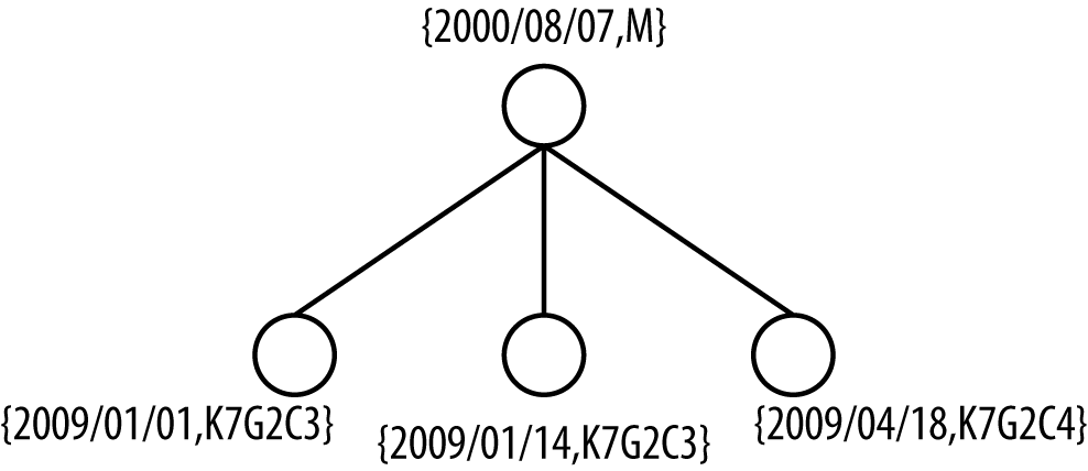
Under the assumption of complete knowledge, we assume that an adversary knows about all of the visits for a specific patient. For PID 10 (Figure 4-2) this means the adversary knows the patient’s date of birth (DOB), gender, the exact dates when he visited the hospital, and where he lived at the time (i.e., his postal code)… stalker! In short, complete knowledge is a worst-case assumption because the adversary knows everything there is to know from the quasi-identifiers. This is a lot of information, but it’s a starting point for developing new ways to assess and manage the risk from longitudinal data. We’ll look at ways of relaxing these assumptions later.

Here’s the problem: we don’t know which patient will be targeted. So there’s no choice but to protect all patients against an adversary with complete knowledge. This means that we have to protect against an adversary with complete knowledge for all patients with one visit, for all patients with two visits, for all patients with three visits… for all patients with any number of visits!

But we do have one saving grace: exact versus approximate complete knowledge. Exact complete knowledge is what we’ve described already. Approximate complete knowledge gives us some leeway because the quasi-identifier values are treated as independent sets. For PID 10, the adversary would know the visit dates {2009/01/01, 2009/01/14, 2009/04/18} and postal codes {K7G2C3, K7G2C3, K7G2C4}, but not which postal codes go with which visit dates. “Approximate” here means that the adversary has all the pieces of information, but doesn’t know how they are connected to each other in visits.

This might seem extreme. How can an adversary that knows dates of visits not know where the target lives? But keep in mind that this is already a lot of information to know about someone. Maybe the adversary knows that the target has moved around a few times, perhaps to a new neighborhood and then back because they preferred the old neighborhood. Maybe the adversary worked at a café near the clinic where the target was seeking treatment, and they’ve chatted. So she knows a lot, but has forgotten how to piece all that information together. The point, rather, is to relax the very strict and conservative assumptions of exact complete knowledge. But if we don’t like an assumption, and we want to connect dates to postal codes even for approximate complete knowledge, we most certainly can.

Connected Variables

There are times when you need to connect variables during de-identification so that they’re treated more or less the same. We consider two basic types of connections:

QI to QI

Sometimes quasi-identifiers are so similar that their de-identification needs to be connected so that both are generalized and suppressed in the same way. Date of delivery and maternal date of discharge are connected because they are strongly correlated—discharge is usually two days after delivery. This means that if you know one you can accurately predict the other. You wouldn’t want one of these dates to be given in weeks and the other in months, which could happen if the two variables weren’t explicitly connected. Another example would be the date of a clinic visit and the date in the log file from an electronic medical record. These two dates will likely be exactly the same because entries in the medical record will happen on the date of the visit. Typically you would connect QIs that are of the same type so that generalizations will be linked and done in the same way.

QI to non-QI

Many quasi-identifiers are coded in some way (e.g., 1 for natural childbirth, 2 for Cesarean), and include a description field to explain what the codes mean without having to look elsewhere. Suppressing the coded value but not the accompanying description would be no different than not doing any suppression at all! Clearly these two fields need to be connected so that suppression is done on both. We see this type of connectedness often in data, with diagnosis, procedure, and drug codes, not to mention any site-specific custom codes. Without a description field these codes become almost meaningless because there are literally thousands of them.

In general, approximate complete knowledge is probably more practical, because exact complete knowledge is so very strong an assumption. Both could be tried as a form of sensitivity analysis to determine their impact on the data. Which one you assume may ultimately depend on how conservative you want to be while preserving data quality. Assuming even approximate complete knowledge may actually be too strong an assumption if there are a significant number of visits, but that’s something we’ll discuss in a later chapter. First let’s look at these concepts in more detail.

Approximate Complete Knowledge

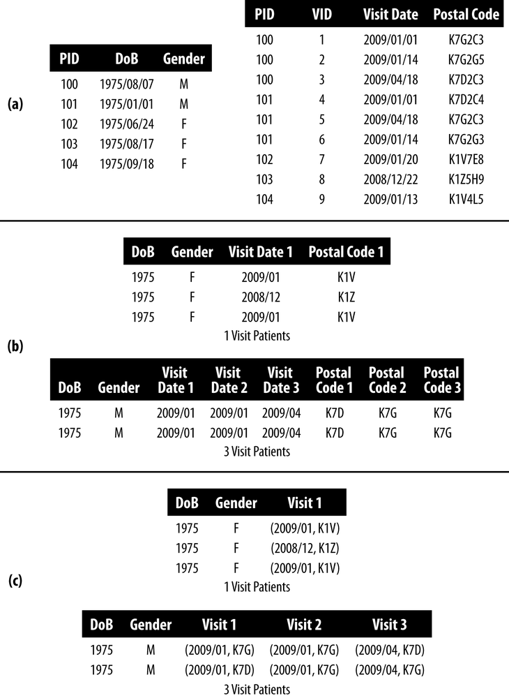
Let’s consider a new data set, given in panel (a) of Figure 4-3. We’ll group patients by the number of visits they had, and flatten the data so each patient is in one row. We’ve done this in panel (b), and performed some generalization to get us close to 2-anonymity. Structuring the data as a series of flat files, based on the number of visits, allows us to use k-anonymity. After all, we don’t want to throw out the baby with the bathwater!

Our generalization in panel (b) got us close to 2-anonymity:

One-visit patients

The first and third patients make an equivalence class of size 2, and the second patient has to be flagged for suppression because she is in an equivalence class of size 1.

Three-visit patients

The visits and postal codes are ordered. The two patients match exactly, creating an equivalence class of size 2.

For approximate complete knowledge, we assume that the adversary doesn’t know which combinations of visit date and postal code go together. An adversary might know, for instance, that the first patient was born in 1975, had two visits in 2009/01 and a visit in 2009/04, and lived at K7D for one visit and at K7G for two visits.

Figure 4-3. The original data (a) under approximate complete knowledge (b) and exact complete knowledge (c)

Exact Complete Knowledge

If we assume exact complete knowledge, we still want to group patients by the number of visits they had and flatten the data so each patient is in one row. But this time, in panel (c) of Figure 4-3, we keep the visit dates and postal codes together as pairs. So, we’re keeping the visit data together before we apply k-anonymity.

Our generalization in panel (c) is the same as before, and gets us close to 2-anonymity:

One-visit patients

The results are the same as before—the second patient has to be flagged for suppression.

Three-visit patients

This time patients don’t match on the first and third visits, because of the postal codes. Both patients therefore have to be flagged for suppression.

Exact complete knowledge is a stricter assumption, leading to more de-identification. In our example, two more patients had to be flagged for suppression than with approximate complete knowledge.

If the longitudinal patterns were more similar, or homogeneous, there would be less difference between exact and approximate knowledge. For example, if patients didn’t move, then their postal codes wouldn’t change, and there would be much less to de-identify. On the flip side, if the longitudinal patterns were less similar, or heterogeneous, there would be a greater difference between exact and approximate knowledge.

Implementation

The implementation of the k-anonymity checks described in the previous sections would not require the creation of multiple tables in practice (i.e., one table for each number of visits). For approximate complete knowledge, each of the values would be represented by its hash value (a hash is a really fast way to identify and filter duplicate information). This would speed up the comparisons of values to compute equivalence classes, and where the values need to be ordered for comparison (for patients with more than one visit), the ordering is performed on the hash values as well. The actual ordering chosen does not actually matter as long as the ordering is performed consistently for all patient records.

The level 2 values for the three-visit patients in panel (b) of Figure 4-3 are ordered by year for dates and alphabetically for postal codes. When hashed, the ordering would be on the hashed values and this would give the same result. An alternative would be to use a commutative hash function, in which case the order would not matter.

Generalization Under Complete Knowledge

The demographics at level 1, DOB and gender, are generalized in the same way as for cross-sectional data, using a generalization hierarchy (like we saw in BORN Data Set). The visit information at level 2, date, and postal code, is generalized in the same way for all visits in the data set. If we generalize the visit date to the year of visit, all of the visit dates for all patients would be generalized to year.

The State Inpatient Database (SID) of California

State Inpatient Databases (SIDs) were developed as part of the Healthcare Cost and Utilization Project (HCUP), a partnership to inform decision making at all levels of government.^[56] All inpatient discharges are collected and abstracted into a uniform format so that one massive database can be created for a participating state. Clinical and nonclinical information is collected from all patients regardless of insurance or lack thereof. It’s a big undertaking with big gains to be had. We only used the 2007 SID of California for this chapter. Some of the more than 100 variables include:

• Patient demographics
• Patient location
• Principal and secondary diagnoses and procedures
• Admission and discharge dates and types
• Length of stay
• Days in intensive care or cardiac care
• Insurance and charges

The SID of California and Open Data

A data use agreement has to be signed in order to access the SID, and some amount of de-identification has already been performed on the data. Just the same, it might be useful to have a public version that could be used to train students, prepare research protocols, confirm published results, improve data quality, and who knows what else. For more precise analyses, the SID could be requested in more detail. The public version would be, well, public, so anyone could use the data as fast as they could download it. But as a public data release, the assumption of approximate complete knowledge would be appropriate to use.

We consider only a subset of the data available in the SID for California, shown in Table 4-1, to get an idea of how these assumptions work in practice. We’re particularly interested in the level 2 quasi-identifiers—i.e., the longitudinal data—which in this case is the admission year, days since last service, and length of stay.

Table 4-1. Quasi-identifiers requested by researcher

Level	Field	Description
1	Gender	Patient’s gender
1	BirthYear	Patient’s year of birth
2	AdmissionYear	Year the patient was first admitted
2	DaysSinceLastService	Number of days since the patient’s last medical service
2	LengthOfStay	Number of days the patient was in the hospital

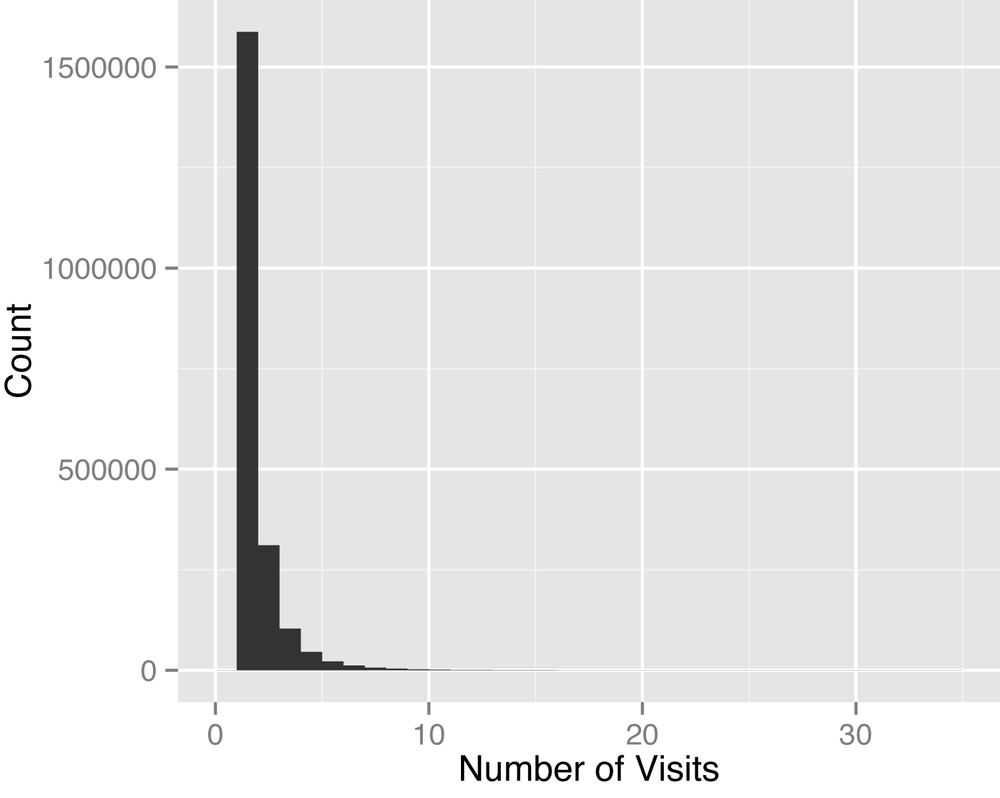
Discharge abstracts are longitudinal, but most patients will only have one or two visits, which means only one or two rows of data per patient. Figure 4-4 captures this best, with a max number of visits of only 34. Of course, a patient that is very sick can have a very long length of stay, but this won’t be captured in the number of visits. Rather, the information for the patient’s stay will be in columns provided in the SID. In Long Tails we’ll see a very different form of longitudinal data, in which each medical claim is captured by a row (so that a long length of stay translates into many rows of data).

Figure 4-4. The short tail of discharge abstracts for the SID of California

The situation is similar to our example using BORN data (see BORN Data Set), except we’re using longitudinal data here. We can’t generalize the gender variable, but a generalization hierarchy was defined for each of the other variables, shown in Table 4-2. Notice that we’re using top and bottom coding in our generalization hierarchy. A bottom code of 1910- for BirthYear means that any year strictly less than 1910 is grouped into “1910-.” These top and bottom codes were necessary due to the distribution of data (it’s never a good idea to blindly apply generalizations to data without first taking a look at it).

Table 4-2. Generalization hierarchy for the quasi-identifiers

Field	Generalization hierarchy
BirthYear	Bottom code 1910-: Year → 5-year interval → 10-year interval
AdmissionYear	Bottom code 2006-: 1-year interval → 2-year interval
DaysSinceLastService	Days up to six, week afterwards, top code 182+ → bottom code 7-, 28-day interval afterwards, top code 182+
LengthOfStay	Connected as to DaysSinceLastService

Risk Assessment

Any researcher, student, or comic book guy can have access to public data. So we have to assume that there’s someone out there that will try to re-identify a record in the data. But we’re not creating a public use file with any sensitive information, so let’s set an overall risk threshold of 0.09 to de-identify the data set, as outlined in Step 2: Setting the Threshold.

Threat Modeling

We only have one plausible attack, as described in Step 3: Examining Plausible Attacks, and it requires us to look at the risk of re-identification in the data set all by itself (i.e., Pr(attempt) = 1, Pr(acquaintance) = 1, and Pr(breach) = 1). We therefore have Pr(re-id) ≤ 0.09, and nothing more. In this case we’ll use maximum risk since we’re talking about a public data set (which is equivalent to k-anonymity with k = 11).

Results

We used approximate complete knowledge to produce a de-identified data set with a minimized amount of cell suppression. Given our generalization hierarchy, the result was a data set with BirthYear bottom code 1910- with 5-year interval, AdmissionYear unchanged, DaysSinceLastService bottom code 7- with 28-day interval and top code 182+, and LengthOfStay the same as DaysSinceLastService because they were connected as QI to QI. Missingness and entropy are shown in Table 4-3 (these are the same measures we first saw in Information Loss Metrics). The results are a first step and can be improved on, as we’ll see in subsequent chapters, but we somewhat expected this given how conservative the assumptions are (with an adversary that knows virtually everything about you… yikes).

Table 4-3. First attempt at de-identification

	Cell missingness	Record missingness	Entropy
Before	0.05%	3.14%
After	15.3%	28.5%	44.7%

We also saw the binary/transactional approach in panel (d) of Figure 4-1, which isn’t actually for longitudinal data but will produce a data set that is properly k-anonymized. As a baseline it will, admittedly, be excessive in its de-identification, but it’s the only viable option for dealing with longitudinal health data under our current set of assumptions. Using approximate complete knowledge on the SID for California, the improvement in entropy was 71.3% compared to this baseline. So we’re getting better, and we’ll look at another adversary model that relaxes these assumptions even further when we get to Chapter 6.

Final Thoughts

Methods developed to de-identify cross-sectional data sets are not appropriate for use on longitudinal data sets. But longitudinal data sets are challenging to de-identify because there can be a lot of information in them. Assuming the adversary knows all will result in de-identified data sets that lose a tremendous amount of their utility. Reasonable assumptions about what an adversary can know need to be made. We’ve discussed some in this chapter, and we have more to come in subsequent chapters. Our purpose here was to get you started on the methods that are needed to deal with more complex data sets.

---

^[48] Schoenman J, Sutton J, Kintala S, Love D, Maw R: “The Value of Hospital Discharge Databases”, Agency for Healthcare Research and Quality, 2005.

^[49] S. Hooley and l. Sweeney: “Survey of Publicly Available State Health Databases”. Harvard University, 2013.

^[50] Robertson J.: “States’ Hospital Data for Sale Puts Privacy in Jeopardy”. Bloomberg News. June 5, 2013.

^[51] B. Malin, L. Sweeney, E. Newton, “Trail Re-identification: Learning Who You Are From Where You Have Been” (Pittsburgh, PA: Carnegie Mellon University, 2003).

^[52] B. Malin and L. Sweeney, “How (Not) to Protect Genomic Data Privacy in a Distributed Network: Using Trails Re-identification to Evaluate and Design Anonymity Protection Systems,” Journal of Biomedical Informatics 37:3 (2004): 179–192.

^[53] Y. Xu, K. Wang, A. Fu, and P. Yu, “Anonymizing Transaction Databases for Publication,” IEEE Transactions on Knowledge Discovery and Data Mining 23:(2008): 161–174.

^[54] G. Ghinita, Y. Tao, and P. Kalnis, “On the Anonymization of Sparse High-Dimensional Data,” Proceedings of the IEEE International Conference on Data Engineering (ICDE, 2008).

^[55] C. Aggarwal, “On k-Anonymity and the Curse of Dimensionality,” Proceedings of the 31st International Conference on Very Large Data Bases (VLDB Endowment, 2005).

^[56] Healthcare Cost and Utilization Project (HCUP) State Inpatient Databases (SID)