Bandit Algorithms for Website Optimization

Chapter 4. Debugging Bandit Algorithms

Monte Carlo Simulations Are Like Unit Tests for Bandit Algorithms

Even though the last chapter contained a full implementation of the epsilon-Greedy algorithm, it was still a very abstract discussion because the algorithm was never run. The reason for that is simple: unlike standard machine learning tools, bandit algorithms aren’t simply black-box functions you can call to process the data you have lying around — bandit algorithms have to actively select which data you should acquire and analyze that data in real-time. Indeed, bandit algorithms exemplify two types of learning that are not present in standard ML examples: active learning, which refers to algorithms that actively select which data they should receive; and online learning, which refers to algorithms that analyze data in real-time and provide results on the fly.

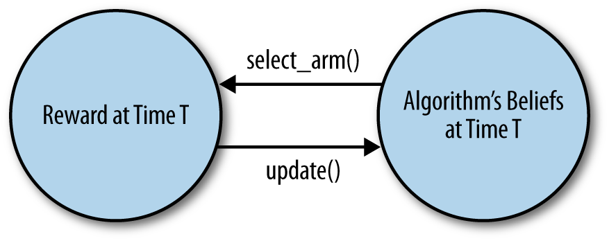
This means that there is a complicated feedback cycle in every bandit algorithm: as shown in Figure 4-1, the behavior of the algorithm depends on the data it sees, but the data the algorithm sees depends on the behavior of the algorithm. Debugging a bandit algorithm is therefore substantially more complicated than debugging a straight machine learning algorithm that isn’t doing active learning. You can’t just feed a bandit algorithm data: you have to turn it loose somewhere to see how it might behave in production. Of course, doing this on your own site could be very risky: you don’t want to unleash untested code on a live site.

Figure 4-1. Bandit data and bandit analysis are inseparable

In order to solve both of these problems, we’re going to use an alternative to standard unit-testing that’s appropriate for testing bandit algorithms. This alternative is called Monte Carlo simulations. The name comes from World War II, when scientists tested how weaponry and other systems might behave by using simple computers equipped with a random number generator.

For our purposes, a Monte Carlo simulation will let our implementation of a bandit algorithm actively make decisions about which data it will receive, because our simulations will be able to provide simulated data in real-time to the algorithm for analysis. In short, we’re going to deal with the feedback cycle shown earlier by coding up both our bandit algorithm and a simulation of the bandit’s arms that the algorithm has to select between. The two pieces of code then work together to generate an example of how the algorithm might really function in production.

Because each simulation is powered by random numbers, the results are noisy. For that reason, you’ll want to run lots of simulations. Thankfully, modern computers, unlike those used in World War II, are well up to the task. As you’ll see in a moment, we can easily simulate 100,000’s of runs of a bandit algorithm to develop an intuition for its behavior in different settings. This is arguably far more important than understanding any specific bandit algorithm, so please don’t skip this section of the book.

Simulating the Arms of a Bandit Problem

In order to reasonably simulate what might happen if you were to deploy an epsilon-Greedy algorithm in production, we need to set up some hypothetical arms. For this book, we’re going to focus on a very simple type of simulated arm that’s easy to implement correctly. This hypothetical arm will let us simulate settings like:

• Optimizing click-through rates for ads: Every time we show someone an ad, we’ll imagine that there’s a fixed probability that they’ll click on the ad. The bandit algorithm will then estimate this probability and try to decide on a strategy for showing ads that maximizes the click-through rate.
• Conversion rates for new users: Every time a new visitor comes to our site who isn’t already a registered user, we’ll imagine that there’s a fixed probability that they’ll register as a user after seeing the landing page. We’ll then estimate this probability and try to decide on a strategy for maximizing our conversion rate.

Our simulated arm is going to be called a Bernoulli arm. Calling this type of an arm a Bernoulli arm is just a jargony way of saying that we’re dealing with an arm that rewards you with a value of 1 some percentage of the time and rewards you with a value of 0 the rest of the time. This 0/1 framework is a very simple way to simulate situations like click-throughs or user signups: the potential user arrives at your site; you select an arm for them in which you, for example, show them one specific color logo; finally, they either do sign up for the site (and give you reward 1) or they don’t (and give you reward 0). If 2% of people who see a red logo sign up and 5% of people who see a green logo sign up, then you can abstract away the details and talk about two arms: one arm outputs 1 unit of reward 2% of the time, the other arm outputs 1 unit of reward 5% of the time. This situation is what we call a Bernoulli arm. We implement it in Python as follows:

class BernoulliArm():
  def __init__(self, p):
    self.p = p

  def draw(self):
    if random.random() > self.p:
      return 0.0
    else:
      return 1.0

First, there’s a class called BernoulliArm that has a single field, p, which tells us the probability of getting a reward of 1 from that arm. Second, there’s a method, draw, that, when called, produces 1 unit of reward with probability p. That’s the entirety of our abstract way of thinking about click-throughs and so on. Amazingly enough, this provides enough material for a very powerful simulation framework.

The only big thing that’s missing from this approach is that we typically have to work with many arms, so we’ll need to set up an array of Arm objects. For example, we could do the following:

means = [0.1, 0.1, 0.1, 0.1, 0.9]
n_arms = len(means)
random.shuffle(means)
arms = map(lambda (mu): BernoulliArm(mu), means)

This will set up an array that contains 5 arms. 4 of them output reward 10% of the time, while the best of them outputs a reward 90% of the time. This is a very black-and-white situation that you won’t see in the real world, but that means that it’s a nice starting point for testing our algorithms. We’ll be using it throughout the rest of this book.

To try out our Bernoulli arms, you might call draw a few times on some of the elements of our array as follows:

arms[0].draw()
arms[1].draw()
arms[2].draw()
arms[2].draw()
arms[3].draw()
arms[2].draw()
arms[4].draw()

A typical output from this might look like:

>>> arms[0].draw()
1.0
>>> arms[1].draw()
0.0
>>> arms[2].draw()
0.0
>>> arms[2].draw()
0.0
>>> arms[3].draw()
0.0
>>> arms[2].draw()
0.0
>>> arms[4].draw()
0.0

That should give you some sense of how this setup works. Our Multiarmed Bandit problem gets represented as an array of arm objects, each of which implements a draw method that simulates playing that specific arm.

With that in place, we’re almost ready to start experimenting with the epsilon-Greedy algorithm. But before we do that, we’re going to set up a very generic framework for testing an algorithm. This framework is described entirely by the test_algorithm function shown below and will be the only testing tool needed for the rest of this book. Let’s go through it now:

def test_algorithm(algo, arms, num_sims, horizon):
  chosen_arms = [0.0 for i in range(num_sims * horizon)]
  rewards = [0.0 for i in range(num_sims * horizon)]
  cumulative_rewards = [0.0 for i in range(num_sims * horizon)]
  sim_nums = [0.0 for i in range(num_sims * horizon)]
  times = [0.0 for i in range(num_sims * horizon)]

  for sim in range(num_sims):
    sim = sim + 1
    algo.initialize(len(arms))

    for t in range(horizon):
      t = t + 1
      index = (sim - 1) * horizon + t - 1
      sim_nums[index] = sim
      times[index] = t

      chosen_arm = algo.select_arm()
      chosen_arms[index] = chosen_arm

      reward = arms[chosen_arms[index]].draw()
      rewards[index] = reward

      if t == 1:
        cumulative_rewards[index] = reward
      else:
        cumulative_rewards[index] = cumulative_rewards[index - 1] + reward

      algo.update(chosen_arm, reward)

  return [sim_nums, times, chosen_arms, rewards, cumulative_rewards]

How does this framework work?

• We pass in a few objects:

  • A bandit algorithm that we want to test.
  • An array of arms we want to simulate draws from.
  • A fixed number of simultations to run to average over the noise in each simulation.
  • The number of times each algorithm is allowed to pull on arms during each simulation. Any algorithm that’s not terrible will eventually learn which arm is best; the interesting thing to study in a simulation is whether an algorithm does well when it only has 100 (or 100,000) tries to find the best arm.

• The framework then uses these objects to run many independent simulations. For each of these, it:

  • Initializes the bandit algorithm’s settings from scratch so that it has no prior knowledge about which arm is best.

  • Loops over opportunities to pull an arm. On each step of this loop, it:

    • Calls select_arm to see which arm the algorithm chooses.
    • Calls draw on that arm to simulate the result of pulling that arm.
    • Records the amount of reward received by the algorithm and then calls update to let the algorithm process that new piece of information.
• Finally, the testing framework returns a data set that tells us for each simulation which arm was chosen and how well the algorithm did at each point in time. In the code directory associated with this book, there are R scripts that plot out the performance to give you a feel for how these algorithms perform. We won’t step through that code in detail in this book, but it is available online in the same GitHub repository as you’re using for all of the other code for this book. Instead of walking through our graphics code, we’ll show you plots that describe what happens during our simulations and try to make sure you understand the main qualitative properties you should be looking for in the data you’ll get from your own simulations.

To show you how to use this testing framework, we need to pass in a specific algorithm and a specific set of arms. In the code below, we show you what happens when applying the epsilon-Greedy algorithm we implemented earlier against the five Bernoulli arms we defined just a moment ago. For simplicity, we’ve reproduced all of the necessary code below, including redefining the five Bernoulli arms:

execfile("core.py")

import random

random.seed(1)
means = [0.1, 0.1, 0.1, 0.1, 0.9]
n_arms = len(means)
random.shuffle(means)
arms = map(lambda (mu): BernoulliArm(mu), means)
print("Best arm is " + str(ind_max(means)))

f = open("algorithms/epsilon_greedy/standard_results.tsv", "w")

for epsilon in [0.1, 0.2, 0.3, 0.4, 0.5]:
  algo = EpsilonGreedy(epsilon, [], [])
  algo.initialize(n_arms)
  results = test_algorithm(algo, arms, 5000, 250)
  for i in range(len(results[0])):
      f.write(str(epsilon) + "\t")
      f.write("\t".join([str(results[j][i]) for j in range(len(results))]) + "\n")

f.close()

Analyzing Results from a Monte Carlo Study

With the results from our simulation study in hand, we can analyze our data in several different ways to assess the performance of our algorithms.

Approach 1: Track the Probability of Choosing the Best Arm

The first analytic approach, and certainly the simplest, is to keep track of the odds that our algorithm selects the best arm at any given point in time. We need to work with odds for two different reasons: (1) the algorithm uses randomization when choosing which arm to pull and may therefore not select the best arm even after it’s learned which arm is best and (2) the rewards that the algorithm receives are random as well. For those reasons, there is always a chance that the algorithm will not make the best decision on any specific trial.

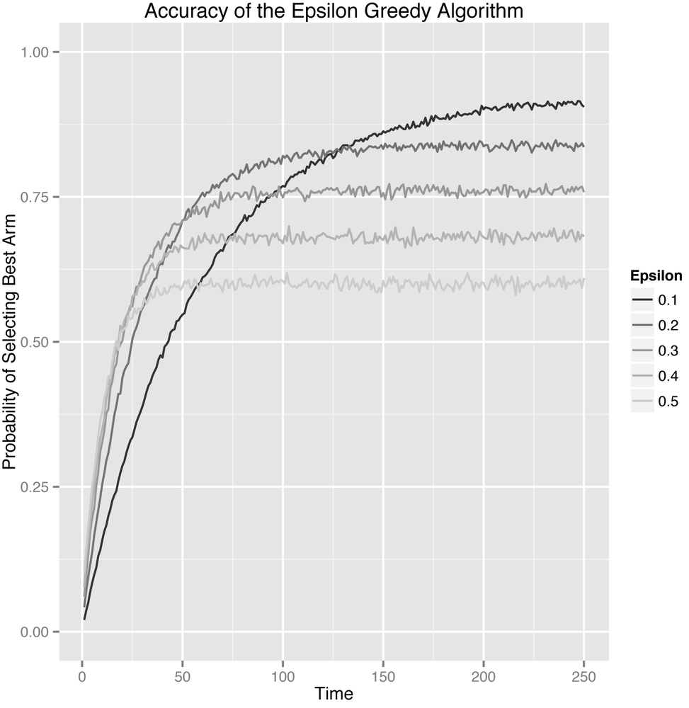
As such, we’ll explicitly calculate the probability of selecting the best arm by estimating the percentage of times in our simulations when the algorithm chose the best arm. If the probability that the algorithm picks the best arm doesn’t go up over time, then we don’t really have any evidence that our algorithm is learning anything about the values of the arms. Thankfully, the results shown in Figure 4-2, which split up the data by the value of epsilon, show that our algorithm does indeed learn no matter how we set epsilon.

Figure 4-2. How often does the algorithm select the best arm?

Let’s step through this graph carefully to understand its message. Before we say anything else, let’s be possibly pedantically clear about the axes:

• The x-axis shows the number of times the algorithm has been able to pull on any of the five arms that are available.
• The y-axis shows the probability that the algorithm, when we called select_arm(), chose the best of the five arms at each point in time.
• The actual values of the curves are the averages across the 5,000 simulations we ran to estimate the algorithm’s performance. We needed to run 5,000 simulations to get around the amount of noise in each simulation caused by using a random number generator in our simulations.

The first thing you should notice is that each setting of epsilon produces a separate curve. The curves with high values of epsilon go up very quickly, but then peak out. That’s a given, because the epsilon-Greedy algorithms choose randomly with probability epsilon. If epsilon is high, we explore a lot and find the best arm quickly, but then we keep exploring even after it’s not worth doing anymore. When epsilon is high, our system’s peak performance is fairly low.

In contrast to the high values of epsilon, the lowest value of epsilon, which was 0.1, causes the algorithm to explore much more slowly, but eventually the algorithm reaches a much higher peak performance level. In many ways, the different settings of epsilon embody the Explore-Exploit trade-off as a whole: the settings that lead to lots of exploration learn quickly, but don’t exploit often enough at the end; whereas the settings that lead to little exploration learn slowly, but do well at the end.

As you can see, which approach is best depends on which point in time you’re looking at. This is why we need to always be concerned about the length of time we intend to leave a bandit algorithm running. The number of pulls that the bandit algorithm has left to it is typically called the horizon. Which algorithm is best depends strongly on the length of the horizon. That will become more clear as we look at other ways of measuring our algorithm’s performance.

Approach 2: Track the Average Reward at Each Point in Time

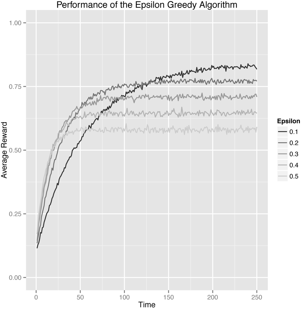
Instead of looking at the probability of picking the best arm, another simple approach to measuring our algorithm’s performance is to use the average reward that our algorithm receives on each trial. When there are many arms similar to the best, each of which is just a little worse than the best, this average reward approach is a much better method of analysis than our approach using probabilities of selecting the best arm. You can see the results for this alternative analysis in Figure 4-3.

Figure 4-3. How much reward does the algorithm earn on average?

In this specific case, the results are quite similar because (A) the rewards are so far apart and because (B) the rewards are all 0’s or 1’s. But these types of metrics can differ much more in other settings. Your mileage may vary.

Approach 3: Track the Cumulative Reward at Each Point in Time

Ultimately, there’s something lacking in both of the approaches we’ve taken: they’re too narrowly focused on the performance of the algorithm at each fixed point in time and don’t give us a gestalt picture of the lifetime performance of our algorithm. This myopic focus on each point in time in isolation is unfair to versions of the epsilon-Greedy algorithm in which epsilon is large, because these algorithms, by definition, explore worse options more frequently than algorithms for which epsilon is low. This is a sacrifice they intentionally make in order to explore faster. To decide whether that increased exploration is worth the trouble, we shouldn’t focus on the performance of the algorithm at any specific point in time, but rather on its cumulative performance over time.

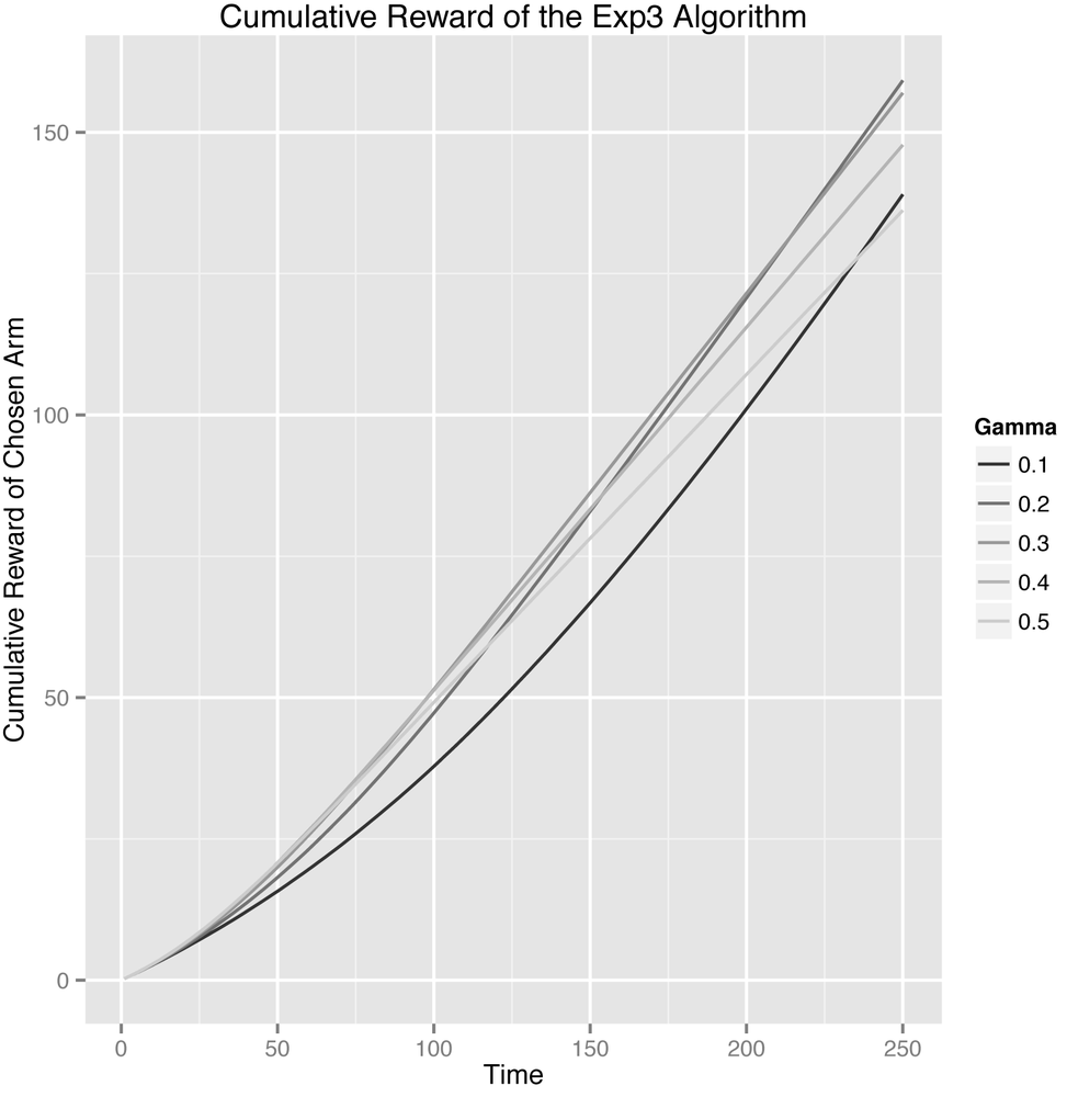
To do that, we can analyze the cumulative reward of our algorithms, which is simply the total amount of reward that an algorithm has won for us up until some fixed point in time. This cumulative reward is important, because it treats algorithms that do a lot of exploration at the start as a means of finding the best available arm more fairly. As you can see in Figure 4-4, an analysis based on cumulative rewards leads to a much cleaner assessment of the performance of the different values of epsilon that we tested.

Figure 4-4. How much reward has the algorithm earned by trial t?

In fact, looking at the cumulative results, you can see that curves for the low value of epsilon = 0.1 and the high value of epsilon = 0.5 intersect after about 130 rounds: before then, it was good to have explored a lot, but after then it was better to have been able to exploit more consistently once the algorithm had found the best arm.

That said, all of our figures convey the same basic message: the epsilon-Greedy algorithm does eventually figure out which arm is best no matter how epsilon is set. But the length of time required to figure our which arm is best depends a lot on the value of epsilon. What’s appropriate for you depends on how long you intend to run your algorithm and how different the arms you’re testing will be. To see how the epsilon-Greedy algorithm might behave for your website, you should use our testing framework to simulate the types of click-through rates you’re used to seeing. We suggest some of these in a list of exercises below.

Exercises

In order to really build a feel for the epsilon-Greedy algorithm, you need to see how it behaves under a variety of circumstances. To do that, you should try out the following exercises:

• Use a different number of arms than the five arms we’ve been working with. See how epsilon-Greedy behaves if there are 2 arms and then see how it behaves if there are 200 arms.
• Change the probabilities of reward from the Bernoulli arms. How does epsilon-Greedy behave if all of the probabilities are close to 0.0? How does it behave it all of the probabilities are close to 1.0? How does it behave when the probabilities for different arms are similar? How does it behave when they’re far apart?

After seeing how the standard epsilon-Greedy algorithm behaves, we’d also encourage you to experiment with trying to modify the epsilon-Greedy to be a little better. There are two specific tricks you will find are worth exploring:

• Change the initialization rules for the values fields. Instead of assuming that every arm has value 0.0 (which amounts to extreme pessimism about unfamiliar arms), try assuming instead that every arm has value 1.0 at the start. How does this change the behavior of the algorithm on different problems?
• Build a modified version of the epsilon-Greedy algorithm that can change the value of epsilon over time, so that epsilon is high at the start and low at the end of a simulation. This change from lots of exploration to little exploration is called annealing and will come up again in the next chapter. Implementing annealing for the epsilon-Greedy algorithm is particularly informative about the weaknesses of the standard epsilon-Greedy algorithm.
• A more involved problem you can work on is to devise an alternative test for evaluting the performance of the epsilon-Greedy algorithm. In this alternative setup, you should keep track of the peformance of the algorithm only on trials when it is trying to exploit. This requires that you store more information during each simulation than we are currently storing, but it can help you to build up an intuition for how the epsilon-Greedy algorithm behaves.