Baseball Hacks

Compare Teams Using Chernoff Faces

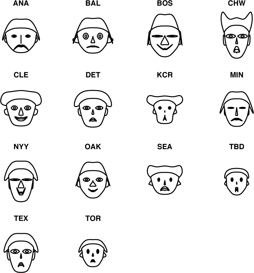
Use your innate ability to recognize facial features to compare teams.

People are naturally very good at recognizing visual patterns, particularly similarities and differences in human faces. In 1973, statistician Herman Chernoff developed a novel technique for comparing data points: plot data points as human faces, where each facial characteristic (mouth size, mouth expression, face shape, eye shape, etc.) represents a different variable in the data. This hack shows you how to apply this idea to baseball teams (or to anything else that you want to compare).

I found two sources of free code for plotting Chernoff faces. The first is from Dr. Hans Peter Wolf. You can find the code on his home page at http://www.wiwi.uni-bielefeld.de/~wolf. The second source is from Shigenobu AOKI, available at http://aoki2.si.gunma-u.ac.jp/R/face.html. In this book, I use Dr. Wolf’s code. (It doesn’t implement the original algorithm exactly, but it’s a lot easier to use.) Just copy all the code from http://www.wiwi.uni-bielefeld.de/~wolf/software/R-wtools/faces/faces.R, paste it into your R window, and hit Return. Or, easier yet, you can just use R’s source() command to load the code in one step. (I show this in the next section.)

Dr. Wolf’s faces() code requires a matrix of values to run. The data in the first column controls the height of the face, the data in the second controls the width, and so on. (See his site for the complete details.) Here are mappings you can use to find teams that are similar offensively:

Table 4-4. 

Column	Facial characteristics	Variable
1	Heightof face	HR
2	Width of face	H
3	Shape of face	HA
4	Height of mouth	HRA
5	Width of mouth	SOA
6	Curve of smile	BB
7	Height of eyes	BBA

As a small wrinkle, the faces() function uses the row names to label the diagram. Because it’s a lot nicer to know which face corresponds to which team than it is to associate row numbers such as “2416,” there’s an extra step to grab the team names. You’ll see this in the code.

The Code

We’ll use an ODBC connection [Hack #33] to the Baseball DataBank database [Hack #10] . Because the SQL statement to select the data spans several lines, the code uses R’s paste() function to concatenate the multiple lines into a single string. Type the following code into R:

	#Load the required libraries
	library(RODBC);

	#Load the faces code
	source("http://www.wiwi.uni-bielefeld.de/~wolf/software/R-wtools/faces/faces.R");

	#Fetch the data that will be used for the faces
	channel<-odbcConnect('bballdata');
	al2003<-sqlQuery(channel, paste (
	  "SELECT HR, H,HA,HRA,SOA,BB, BBA ",
	  "FROM teams WHERE ",
	  "lgID = 'AL' AND ",
	  "yearID = 2003"));
	#Fetch the team names and save as the row names
	row.names(al2003)<- sqlQuery(channel, paste (
	 "SELECT teamID FROM teams WHERE lgID = 'AL' AND yearID = 2003"))$teamID;
	# Run the faces program
	faces(as.matrix(al2003));

Run the Hack

Here’s the al2003 data set that I got when I ran the preceding code:

	>al2003
	     HR    H   HA HRA  SOA  BB BBA
	ANA 150 1473 1444 190  980 476 486
	BAL 152 1516 1579 198  981 431 526
	BOS 238 1667 1503 153 1141 620 488
	CHA 220 1445 1364 162 1056 519 518
	CLE 158 1413 1477 179  943 466 501
	DET 153 1312 1616 195  764 443 557
	KCA 162 1526 1569 190  865 476 566
	MIN 155 1567 1526 187  997 512 402
	NYA 230 1518 1512 145 1119 684 375
	OAK 176 1398 1336 140 1018 556 499
	SEA 139 1509 1340 173 1001 586 466
	TBA 137 1501 1454 196  877 420 639
	TEX 239 1506 1625 208 1009 488 603
	TOR 190 1580 1560 184  984 546 485

Figure 4-14 shows the output of the faces() plot for this data. As you can see, Boston scored many more runs than Baltimore did, so its face is much taller; Texas allowed a lot more home runs than Oakland did, so its mouth is larger.

What I find most remarkable about this diagram is that it’s not total nonsense. For example, the Yankees and the Red Sox are fairly similar offensive teams in many ways, and their “faces” bear out this resemblance.

Hacking the Hack

Here are some ideas for different things to compare with faces():

Compare groups of players

You can easily run this code on other groups of players to try to find similarities. I suggest trying groups of batters and pitchers.

Find players similar in some characteristics

If, for example, you want to look at pitcher injuries and compare similar players, you can use Chernoff faces to find pitchers who are most similar to one another.

Figure 4-14. Chernoff faces