Data Science for Business

Chapter 4. Fitting a Model to Data

Fundamental concepts: Finding “optimal” model parameters based on data; Choosing the goal for data mining; Objective functions; Loss functions.

Exemplary techniques: Linear regression; Logistic regression; Support-vector machines.

As we have seen, predictive modeling involves finding a model of the target variable in terms of other descriptive attributes. In Chapter 3, we constructed a supervised segmentation model by recursively finding informative attributes on ever-more-precise subsets of the set of all instances, or from the geometric perspective, ever-more-precise subregions of the instance space. From the data we produced both the structure of the model (the particular tree model that resulted from the tree induction) and the numeric “parameters” of the model (the probability estimates at the leaf nodes).

An alternative method for learning a predictive model from a dataset is to start by specifying the structure of the model with certain numeric parameters left unspecified. Then the data mining calculates the best parameter values given a particular set of training data. A very common case is where the structure of the model is a parameterized mathematical function or equation of a set of numeric attributes. The attributes used in the model could be chosen based on domain knowledge regarding which attributes ought to be informative in predicting the target variable, or they could be chosen based on other data mining techniques, such as the attribute selection procedures introduced in Chapter 3. The data miner specifies the form of the model and the attributes; the goal of the data mining is to tune the parameters so that the model fits the data as well as possible. This general approach is called parameter learning or parametric modeling.

Note

In certain fields of statistics and econometrics, the bare model with unspecified parameters is called “the model.” We will clarify that this is the structure of the model, which still needs to have its parameters specified to be useful.

Many data mining procedures fall within this general framework. We will illustrate with some of the most common, all of which are based on linear models. If you’ve taken a statistics course, you’re probably already familiar with one linear modeling technique: linear regression. We will see the same differences in models that we’ve seen already, such as the differences in task between classification, class probability estimation, and regression. As examples we will present some common techniques used for predicting (estimating) unknown numeric values, unknown binary values (such as whether a document or web page is relevant to a query), as well as likelihoods of events, such as default on credit, response to an offer, fraud on an account, and so on.

We also will explicitly discuss something that we skirted in Chapter 3: what exactly do we mean when we say a model fits the data well? This is the crux of the fundamental concept of this chapter—fitting a model to data by finding “optimal” model parameters—and is a notion that will resurface in later chapters. Because of its fundamental concepts, this chapter is more mathematically focused than the rest. We will keep the math to a minimum, and encourage the less mathematical reader to proceed boldly.

Sidebar: Simplifying Assumptions in This Chapter

The point of this chapter is to introduce and explain parametric modeling. To keep the discussion focused, and to avoid excessive footnotes, we’ve made some simplifying assumptions:

• First, for classification and class probability estimation we will consider only binary classes: the models predict events that either take place or do not, such as responding to an offer, leaving the company, being defrauded, etc. The methods here can all be generalized to work with multiple (nonbinary) classes, but the generalization complicates the description unnecessarily.
• Second, because we’re dealing with equations, this chapter assumes all attributes are numeric. There are techniques for converting categorical (symbolic) attributes into numerical values for use with these equations.
• Finally, we ignore the need to normalize numeric measurements to a common scale. Attributes such as Age and Income have vastly different ranges and they are usually normalized to a common scale to help with model interpretability, as well as other things (to be discussed later).

We ignore these complications in this chapter. However, dealing with them is ultimately important and often necessary regardless of the data mining technique.

Classification via Mathematical Functions

Figure 4-1. A dataset split by a classification tree with four leaf nodes.

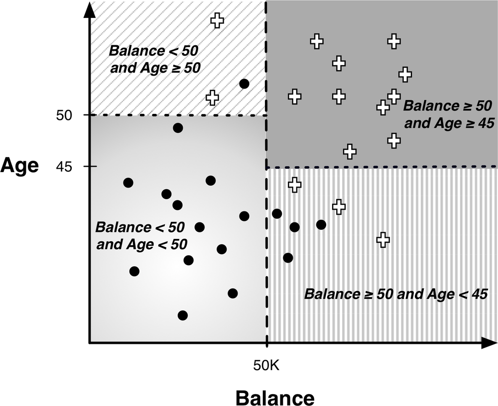
Recall the instance-space view of tree models from Chapter 3. One such diagram is replicated in Figure 4-1. It shows the space broken up into regions by horizontal and vertical decision boundaries that partition the instance space into similar regions. Examples in each region should have similar values for the target variable. In the last chapter we saw how the entropy measure gives us a way of measuring homogeneity so we can choose such boundaries.

A main purpose of creating homogeneous regions is so that we can predict the target variable of a new, unseen instance by determining which segment it falls into. For example, in Figure 4-1, if a new customer falls into the lower-left segment, we can conclude that the target value is very likely to be “•”. Similarly, if it falls into the upper-right segment, we can predict its value as “+”.

Figure 4-2. The raw data points of Figure 4-1, without decision lines.

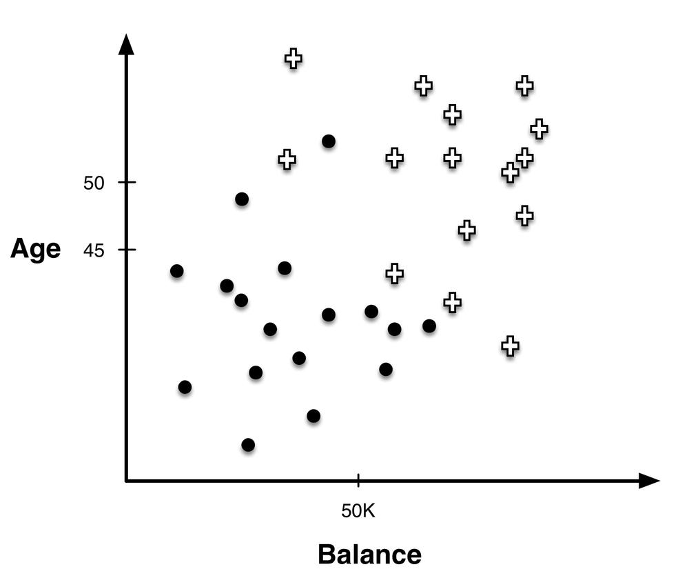
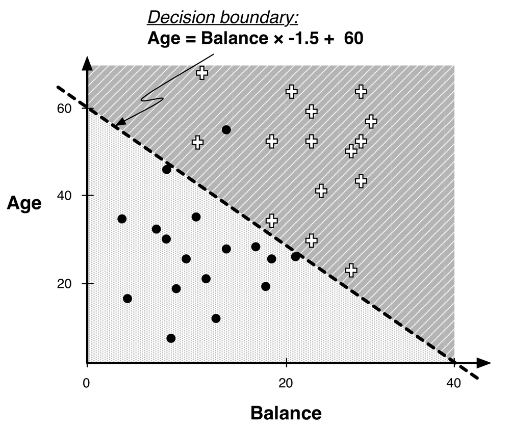
The instance-space view is helpful because if we take away the axis-parallel boundaries (see Figure 4-2) we can see that there clearly are other, possibly better, ways to partition the space. For example, we can separate the instances almost perfectly (by class) if we are allowed to introduce a boundary that is still a straight line, but is not perpendicular to the axes (Figure 4-3).

Figure 4-3. The dataset of Figure 4-2 with a single linear split.

This is called a linear classifier and is essentially a weighted sum of the values for the various attributes, as we will describe next.

Linear Discriminant Functions

Our goal is going to be to fit our model to the data, and to do so it is quite helpful to represent the model mathematically. You may recall that the equation of a line in two dimensions is y = mx + b, where m is the slope of the line and b is the y intercept (the y value when x = 0). The line in Figure 4-3 can be expressed in this form (with Balance in thousands) as:

We would classify an instance x as a + if it is above the line, and as a • if it is below the line. Rearranging this mathematically leads to the function that is the basis of all the techniques discussed in this chapter. For this example decision boundary, the classification solution is shown in Equation 4-1.

Equation 4-1. Classification function

This is called a linear discriminant because it discriminates between the classes, and the function of the decision boundary is a linear combination—a weighted sum—of the attributes. In the two dimensions of our example, the linear combination corresponds to a line. In three dimensions, the decision boundary is a plane, and in higher dimensions it is a hyperplane (see Decision lines and hyperplanes in Visualizing Segmentations). For our purposes, the important thing is that we can express the model as a weighted sum of the attribute values.

Thus, this linear model is a different sort of multivariate supervised segmentation. Our goal with supervised segmentation still is to separate the data into regions with different values of the target variable. The difference is that the method for taking multiple attributes into account is to create a mathematical function of them.

In Trees as Sets of Rules we showed how a classification tree corresponds to a rule set—a logical classification model of the data. A linear discriminant function is a numeric classification model. For example, consider our feature vector x, with the individual component features being x_i. A linear model then can be written as follows in Equation 4-2.

Equation 4-2. A general linear model

The concrete example from Equation 4-1 can be written in this form:

To use this model as a linear discriminant, for a given instance represented by a feature vector x, we check whether f(x) is positive or negative. As discussed above, in the two-dimensional case, this corresponds to seeing whether the instance x falls above or below the line.

Linear functions are one of the workhorses of data science; now we finally come to the data mining. We now have a parameterized model: the weights of the linear function (w_i) are the parameters.^[21] The data mining is going to “fit” this parameterized model to a particular dataset—meaning specifically, to find a good set of weights on the features.

After learning, these weights are often loosely interpreted as importance indicators of the features. Roughly, the larger the magnitude of a feature’s weight, the more important that feature is for classifying the target—assuming all feature values have been normalized to the same range, as mentioned in Sidebar: Simplifying Assumptions in This Chapter. By the same token, if a feature’s weight is near zero the corresponding feature can usually be ignored or discarded. For now, we are interested in a set of weights that discriminate the training data well and predict as accurately as possible the value of the target variable for cases where we don’t know it.

Figure 4-4. A basic instance space in two dimensions containing points of two classes.

Figure 4-5. Many different possible linear boundaries can separate the two groups of points of Figure 4-4.

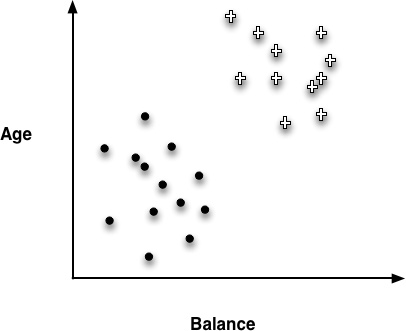
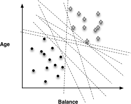
Unfortunately, it’s not trivial to choose the “best” line to separate the classes. Let’s consider a simple case, illustrated in Figure 4-4. Here the training data can indeed be separated by class using a linear discriminant. However, as shown in Figure 4-5, there actually are many different linear discriminants that can separate the classes perfectly. They have very different slopes and intercepts, and each represents a different model of the data. In fact, there are infinitely many lines (models) that classify this training set perfectly. Which should we pick?

Optimizing an Objective Function

This brings us to one of the most important fundamental ideas in data mining—one that surprisingly is often overlooked even by data scientists themselves: we need to ask, what should be our goal or objective in choosing the parameters? In our case, this would allow us to answer the question: what weights should we choose? Our general procedure will be to define an objective function that represents our goal, and can be calculated for a particular set of weights and a particular set of data. We will then find the optimal value for the weights by maximizing or minimizing the objective function. What can easily be overlooked is that these weights are “best” only if we believe that the objective function truly represents what we want to achieve, or practically speaking, is the best proxy we can come up with. We will return to this later in the book.

Unfortunately, creating an objective function that matches the true goal of the data mining is usually impossible, so data scientists often choose based on faith^[22] and experience. Several choices have been shown to be remarkably effective. One of these choices creates the so-called “support vector machine,” about which we will say a few words after presenting a concrete example with a simpler objective function. After that, we will briefly discuss linear models for regression, rather than classification, and end with one of the most useful data mining techniques of all: logistic regression. Its name is something of a misnomer—logistic regression doesn’t really do what we call regression, which is the estimation of a numeric target value. Logistic regression applies linear models to class probability estimation, which is particularly useful for many applications.

Linear regression, logistic regression, and support vector machines are all very similar instances of our basic fundamental technique: fitting a (linear) model to data. The key difference is that each uses a different objective function.

An Example of Mining a Linear Discriminant from Data

To illustrate linear discriminant functions, we use an adaptation of the Iris dataset taken from the UCI Dataset Repository (Bache & Lichman, 2013). This is an old and fairly simple dataset representing various types of iris, a genus of flowering plant. The original dataset includes three species of irises represented with four attributes, and the data mining problem is to classify each instance as belonging to one of the three species based on the attributes.

Figure 4-6. Two parts of a flower. Width measurements of these are used in the Iris dataset.

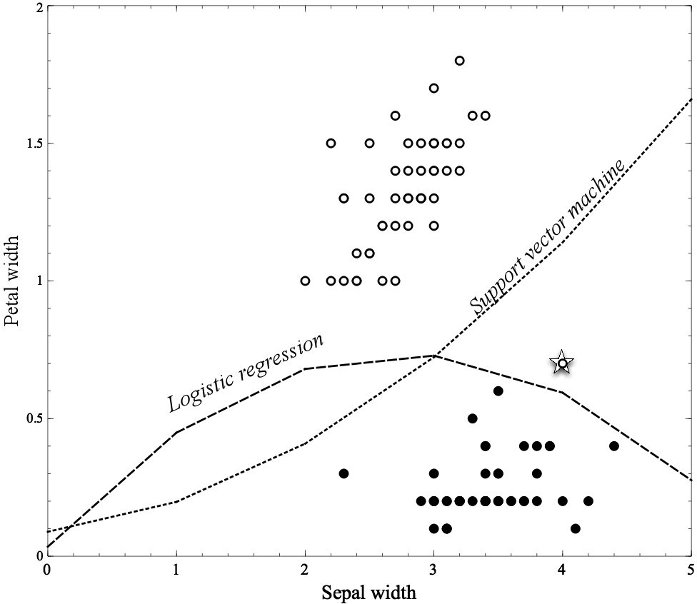
For this illustration we’ll use just two species of irises, Iris Setosa and Iris Versicolor. The dataset describes a collection of flowers of these two species, each described with two measurements: the Petal width and the Sepal width (Figure 4-6). The flower dataset is plotted in Figure 4-7, with these two attributes on the x and y axis, respectively. Each instance is one flower and corresponds to one dot on the graph. The filled dots are of the species Iris Setosa and the circles are instances of the species Iris Versicolor.

Figure 4-7. A dataset and two learned linear classifiers.

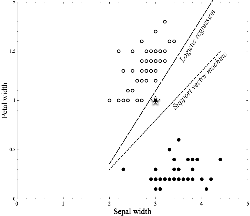
Two different separation lines are shown in the figure, one generated by logistic regression and the second by another linear method, a support vector machine (which will be described shortly). Note that the data comprise two fairly distinct clumps, with a few outliers. Logistic regression separates the two classes completely: all the Iris Versicolor examples are to the left of its line and all the Iris Setosa to the right. The Support vector machine line is almost midway between the clumps, though it misclassifies the starred point at (3, 1).^[23] Which separator do you think is better? In Chapter 5, we will get into details of why these separators are different and why one might be preferable to the other. For now it’s enough just to notice that the methods produce different boundaries because they’re optimizing different functions.

Linear Discriminant Functions for Scoring and Ranking Instances

In many applications, we don’t simply want a yes or no prediction of whether an instance belongs to the class, but we want some notion of which examples are more or less likely to belong to the class. For example, which consumers are most likely to respond to this offer? Which customers are most likely to leave when their contracts expire? One option is to build a model that produces an estimate of class membership probability, as we did with tree induction for class probability estimation in Chapter 3. We can do this with linear models as well, and will treat this in detail below when we introduce logistic regression.

In other applications, we do not need a precise probability estimate. We simply need a score that will rank cases by the likelihood of belonging to one class or the other. For example, for targeted marketing we may have a limited budget for targeting prospective customers. We would like to have a list of consumers ranked by their predicted likelihood of responding positively to our offer. We don’t necessarily need to be able to estimate the exact probability of response accurately, as long as the list is ranked reasonably well, and the consumers at the top of the list are the ones most likely to respond.

Linear discriminant functions can give us such a ranking for free. Look at Figure 4-4, and consider the + instances to be responders and • instances to be nonresponders. Assume we are presented with a new instance x for which we do not yet know the class (i.e., we have not yet made an offer to x). In which portion of the instance space would we like x to fall in order to expect the highest likelihood of response? Where would we be most certain that x would not respond? Where would we be most uncertain?

Many people suspect that right near the decision boundary we would be most uncertain about a class (and see the discussion below on the “margin”). Far away from the decision boundary, on the + side, would be where we would expect the highest likelihood of response. In the equation of the separating boundary, given above in Equation 4-2, f(x) will be zero when x is sitting on the decision boundary (technically, x in that case is one of the points of the line or hyperplane). f(x) will be relatively small when x is near the boundary. And f(x) will be large (and positive) when x is far from the boundary in the + direction. Thus f(x) itself—the output of the linear discriminant function—gives an intuitively satisfying ranking of the instances by their (estimated) likelihood of belonging to the class of interest.

Support Vector Machines, Briefly

If you’re even on the periphery of the world of data science these days, you eventually will run into the support vector machine or “SVM.” This is a notion that can strike fear into the hearts even of people quite knowledgeable in data science. Not only is the name itself opaque, but the method often is imbued with the sort of magic that derives from perceived effectiveness without understanding.

Fortunately, we now have the concepts necessary to understand support vector machines. In short, support vector machines are linear discriminants. For many business users interacting with data scientists, that will be sufficient. Nevertheless, let’s look at SVMs a little more carefully; if we can get through some minor details, the procedure for fitting the linear discriminant is intuitively satisfying.

As with linear discriminants generally, SVMs classify instances based on a linear function of the features, described above in Equation 4-2.

Note

You may also hear of nonlinear support vector machines. Oversimplifying slightly, a nonlinear SVM uses different features (that are functions of the original features), so that the linear discriminant with the new features is a nonlinear discriminant with the original features.

So, as we’ve discussed, the crucial question becomes: what is the objective function that is used to fit an SVM to data? For now we will skip the mathematical details in order to gain an intuitive understanding. There are two main ideas.

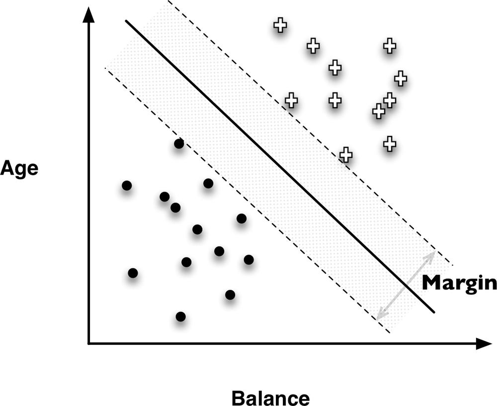
Recall Figure 4-5 showing the infinitude of different possible linear discriminants that would separate the classes, and recall that choosing an objective function for fitting the data amounts to choosing which of these lines is the best. SVMs choose based on a simple, elegant idea: instead of thinking about separating with a line, first fit the fattest bar between the classes. This is shown by the parallel dashed lines in Figure 4-8.

The SVM’s objective function incorporates the idea that a wider bar is better. Then once the widest bar is found, the linear discriminant will be the center line through the bar (the solid middle line in Figure 4-8). The distance between the dashed parallel lines is called the margin around the linear discriminant, and thus the objective is to maximize the margin.

Figure 4-8. The points of Figure 4-2 and the maximal margin classifier.

The idea of maximizing the margin is intuitively satisfying for the following reason. The training dataset is just a sample from some population. In predictive modeling, we are interested in predicting the target for instances that we have not yet seen. These instances will be scattered about. Hopefully they will be distributed similarly to the training data, but they will in fact be different points. In particular, some of the positive examples will likely fall closer to the discriminant boundary than any positive example we have yet seen. All else being equal, the same applies to the negative examples. In other words, they may fall in the margin. The margin-maximizing boundary gives the maximal leeway for classifying such points. Specifically, by choosing the SVM decision boundary, in order for a new instance to be misclassified, one would have to place it further into the margin than with any other linear discriminant. (Or, of course, completely on the wrong side of the margin bar altogether.)

The second important idea of SVMs lies in how they handle points falling on the wrong side of the discrimination boundary. The original example of Figure 4-2 shows a situation in which a single line cannot perfectly separate the data into classes. This is true of most data from complex real-world applications—some data points will inevitably be misclassified by the model. This does not pose a problem for the general notion of linear discriminants, as their classifications don’t necessarily have to be correct for all points. However, when fitting the linear function to the data we cannot simply ask which of all the lines that separate the data perfectly should we choose. There may be no such perfect separating line!

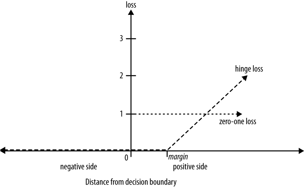
Once again, the support-vector machine’s solution is intuitively satisfying. Skipping the math, the idea is as follows. In the objective function that measures how well a particular model fits the training points, we will simply penalize a training point for being on the wrong side of the decision boundary. In the case where the data indeed are linearly separable, we incur no penalty and simply maximize the margin. If the data are not linearly separable, the best fit is some balance between a fat margin and a low total error penalty. The penalty for a misclassified point is proportional to the distance from the margin boundary, so if possible the SVM will make only “small” errors. Technically, this error function is known as hinge loss (see Sidebar: Loss functions and Figure 4-9).

Figure 4-9. Two loss functions illustrated. The x axis shows the distance from the decision boundary. The y axis shows the loss incurred by a negative instance as a function of its distance from the decision boundary. (The case of a positive instance is symmetric.) If the negative instance is on the negative side of the boundary, there is no loss. If it is on the positive (wrong) side of the boundary, the different loss functions penalize it differently. (See Sidebar: Loss functions.)

Regression via Mathematical Functions

The previous chapter introduced the fundamental notion of selecting informative variables. We showed that this notion applies to classification, to regression, and to class probability estimation. Here too, this chapter’s basic notion of fitting linear functions to data applies to classification, regression, and to class probability estimation. Let’s now discuss regression briefly.^[24]

Sidebar: Loss functions

The term “loss” is used across data science as a general term for error penalty. A loss function determines how much penalty should be assigned to an instance based on the error in the model’s predicted value—in our present context, based on its distance from the separation boundary. Several loss functions are commonly used (two are shown in Figure 4-9). In the figure, the horizontal axis is the distance from the separating boundary. Errors have positive distances from the separator in Figure 4-9, while correct classifications have negative distances (the choice is arbitrary in this diagram).

Support vector machines use hinge loss, so called because the loss graph looks like a hinge. Hinge loss incurs no penalty for an example that is not on the wrong side of the margin. The hinge loss only becomes positive when an example is on the wrong side of the boundary and beyond the margin. Loss then increases linearly with the example’s distance from the margin, thereby penalizing points more the farther they are from the separating boundary.

Zero-one loss, as its name implies, assigns a loss of zero for a correct decision and one for an incorrect decision.

For contrast, consider a different sort of loss function. Squared error specifies a loss proportional to the square of the distance from the boundary. Squared error loss usually is used for numeric value prediction (regression), rather than classification. The squaring of the error has the effect of greatly penalizing predictions that are grossly wrong. For classification, this would apply large penalties to points far over on the “wrong side” of the separating boundary. Unfortunately, using squared error for classification also penalizes points far on the correct side of the decision boundary. For most business problems, choosing squared-error loss for classification or class-probability estimation thus would violate our principle of thinking carefully about whether the loss function is aligned with the business goal. (Hinge-like versions of squared error have been created because of this misalignment [Rosset & Zhu, 2007].)

We have already discussed most of what we need for linear regression. The linear regression model structure is exactly the same as for the linear discriminant function Equation 4-2:

So, following our general framework for thinking about parametric modeling, we need to decide on the objective function we will use to optimize the model’s fit to the data. There are many possibilities. Each different linear regression modeling procedure uses one particular choice (and the data scientist should think carefully about whether it is appropriate for the problem).

The most common (“standard”) linear regression procedure makes a powerful and convenient choice. Recall that for regression problems the target variable is numeric. The linear function estimates this numeric target value using Equation 4-2, and of course the training data have the actual target value. Therefore, an intuitive notion of the fit of the model is: how far away are the estimated values from the true values on the training data? In other words, how big is the error of the fitted model? Presumably we’d like to minimize this error. For a particular training dataset, we could compute this error for each individual data point and sum up the results. Then the model that fits the data best would be the model with the minimum sum of errors on the training data. And that is exactly what regression procedures do.

You might notice that we really have not actually specified the objective function, because there are many ways to compute the error between an estimated value and an actual value. The method that is most natural is to simply subtract one from the other (and take the absolute value). So if I predict 10 and the actual value is 12 or 8, I make an error of 2. This is called absolute error, and we could then minimize the sum of absolute errors or equivalently the mean of the absolute errors across the training data. This makes a lot of sense, but it is not what standard linear regression procedures do.

Standard linear regression procedures instead minimize the sum or mean of the squares of these errors—which gives the procedure its common name “least squares” regression. So why do so many people use least squares regression without much thought to alternatives? The short answer is convenience. It is the technique we learn in basic statistics classes (and beyond). It is available to us to use in various software packages. Originally, the least squared error function was introduced by the famous 18th century mathematician Carl Friedrich Gauss, and there are certain theoretical arguments for its use (relating to the normal or “Gaussian” distribution). Often, more importantly, it turns out that squared error is particularly convenient mathematically.^[25] This was helpful in the days before computers. From a data science perspective, the convenience extends to theoretical analyses, including a clean decomposition of model error into different sources. More pragmatically, analysts often claim to prefer squared error because it strongly penalizes very large errors. Whether the quadratic penalty is actually appropriate is specific to each application. (Why not take the fourth power of the errors, and penalize large errors even more strongly?)

Importantly, any choice for the objective function has both advantages and drawbacks. For least squares regression a serious drawback is that it is very sensitive to the data: erroneous or otherwise outlying data points can severely skew the resultant linear function. For some business applications, we may not have the resources to spend as much time on manual massaging of the data as we would in other applications. At the extreme, for systems that build and apply models totally automatically, the modeling needs to be much more robust than when doing a detailed regression analysis “by hand.” Therefore, for the former application we may want to use a more robust modeling procedure (e.g., use as the objective function absolute error instead of squared error). An important thing to remember is that once we see linear regression simply as an instance of fitting a (linear) model to data, we see that we have to choose the objective function to optimize—and we should do so with the ultimate business application in mind.

Class Probability Estimation and Logistic “Regression”

As mentioned earlier, for many applications we would like to estimate the probability that a new instance belongs to the class of interest. In many cases, we would like to use the estimated probability in a decision-making context that includes other factors such as costs and benefits. For example, predictive modeling from large consumer data is used widely in fraud detection across many industries, especially banking, telecommunications, and online commerce. A linear discriminant could be used to identify accounts or transactions as likely to have been defrauded. The director of the fraud control operation may want the analysts to focus not simply on the cases most likely to be fraud, but on the cases where the most money is at stake—that is, accounts where the company’s monetary loss is expected to be the highest. For this we need to estimate the actual probability of fraud. (Chapter 7 will discuss in detail the use of expected value to frame business problems.)

Fortunately, within this same framework for fitting linear models to data, by choosing a different objective function we can produce a model designed to give accurate estimates of class probability. The most common procedure by which we do this is called logistic regression.

Note

What exactly is an accurate estimate of class membership probability is a subject of debate beyond the scope of this book. Roughly, we would like (i) the probability estimates to be well calibrated, meaning that if you take 100 cases whose class membership probability is estimated to be 0.2, then about 20 of them will actually belong to the class. We would also like (ii) the probability estimates to be discriminative, in that if possible they give meaningfully different probability estimates to different examples. The latter condition keeps us from simply giving the “base rate” (the overall prevalence in the population) as the prediction for every example. Say 0.5% of accounts overall are fraudulent. Without condition (ii) we could simply predict the same 0.5% probability for each account; those estimates would be well calibrated—but not discriminative at all.

To understand logistic regression, it is instructive to first consider: exactly what is the problem with simply using our basic linear model (Equation 4-2) to estimate the class probability? As we discussed, an instance being further from the separating boundary intuitively ought to lead to a higher probability of being in one class or the other, and the output of the linear function, f(x), gives the distance from the separating boundary. However, this also shows the problem: f(x) ranges from –∞ to ∞, and a probability should range from zero to one.

So let’s take a brief stroll down a garden path and ask how else we might cast our distance from the separator, f(x), in terms of the likelihood of class membership. Is there another representation of the likelihood of an event that we use in everyday life? If we could come up with one that ranges from –∞ to ∞, then we might model this other notion of likelihood with our linear equation.

One very useful notion of the likelihood of an event is the odds. The odds of an event is the ratio of the probability of the event occurring to the probability of the event not occurring. So, for example, if the event has an 80% probability of occurrence, the odds are 80:20 or 4:1. And if the linear function were to give us the odds, a little algebra would tell us the probability of occurrence. Let’s look at a more detailed example. Table 4-1 shows the odds corresponding to various probabilities.

Table 4-1. Probabilities and the corresponding odds.

Probability	Corresponding odds
0.5	50:50 or 1
0.9	90:10 or 9
0.999	999:1 or 999
0.01	1:99 or 0.0101
0.001	1:999 or 0.001001

Looking at the range of the odds in Table 4-1, we can see that it still is not quite right as an interpretation of the distance from the separating boundary. Again, the distance from the boundary is between –∞ and ∞, but as we can see from the example, the odds range from 0 to ∞. Nonetheless, we can solve our garden-path problem simply by taking the logarithm of the odds (called the “log-odds”), since for any number in the range 0 to ∞ its log will be between –∞ to ∞. These are shown in Table 4-2.

Table 4-2. Probabilities, odds, and the corresponding log-odds.

Probability	Odds	Log-odds
0.5	50:50 or 1	0
0.9	90:10 or 9	2.19
0.999	999:1 or 999	6.9
0.01	1:99 or 0.0101	–4.6
0.001	1:999 or 0.001001	–6.9

So if we only cared about modeling some notion of likelihood, rather than the class membership probability specifically, we could model the log-odds with f(x).

Lo and behold, our garden path has taken us directly back to our main topic. This is exactly a logistic regression model: the same linear function f(x) that we’ve examined throughout the chapter is used as a measure of the log-odds of the “event” of interest. More specifically, f(x) is the model’s estimation of the log-odds that x belongs to the positive class. For example, the model might estimate the log-odds that a customer described by feature vector x will leave the company when her contract expires. Moreover, with a little algebra we can translate these log-odds into the probability of class membership. This is a little more technical than most of the book, so we’ve relegated it to a special “technical details” subsection (next), which also discusses what exactly is the objective function that is optimized to fit a logistic regression to the data. You can read that section in detail or just skim it. The most important points are:

• For probability estimation, logistic regression uses the same linear model as do our linear discriminants for classification and linear regression for estimating numeric target values.
• The output of the logistic regression model is interpreted as the log-odds of class membership.
• These log-odds can be translated directly into the probability of class membership. Therefore, logistic regression often is thought of simply as a model for the probability of class membership. You have undoubtedly dealt with logistic regression models many times without even knowing it. They are used widely to estimate quantities like the probability of default on credit, the probability of response to an offer, the probability of fraud on an account, the probability that a document is relevant to a topic, and so on.

After the technical details section, we will compare the linear models we’ve developed in this chapter with the tree-structured models we developed in Chapter 3.

Note: Logistic regression is a misnomer

Above we mentioned that the name logistic regression is a misnomer under the modern use of data science terminology. Recall that the distinction between classification and regression is whether the value for the target variable is categorical or numeric. For logistic regression, the model produces a numeric estimate (the estimation of the log-odds). However, the values of the target variable in the data are categorical. Debating this point is rather academic. What is important to understand is what logistic regression is doing. It is estimating the log-odds or, more loosely, the probability of class membership (a numeric quantity) over a categorical class. So we consider it to be a class probability estimation model and not a regression model, despite its name.

* Logistic Regression: Some Technical Details

Technical Details Ahead

Since logistic regression is used so widely, and is not as intuitive as linear regression, let’s examine a few of the technical details. You may skip this subsection without it affecting your understanding of the rest of the book.

So, technically, what is the bottom line for the logistic regression model?

Let’s use to represent the model’s estimate of the probability of class membership of a data item represented by feature vector x.^[26] Recall that the class + is whatever is the (binary) event that we are modeling: responding to an offer, leaving the company after contract expiration, being defrauded, etc. The estimated probability of the event not occurring is therefore .

Equation 4-3. Log-odds linear function

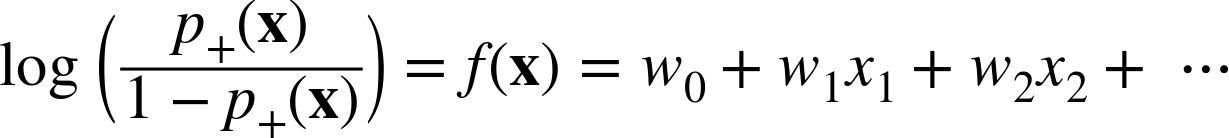
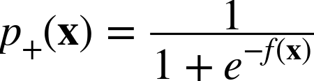
Thus, Equation 4-3 specifies that for a particular data item, described by feature-vector x, the log-odds of the class is equal to our linear function, f(x). Since often we actually want the estimated probability of class membership, not the log-odds, we can solve for in Equation 4-3. This yields the not-so-pretty quantity in Equation 4-4.

Equation 4-4. The logistic function

Although the quantity in Equation 4-4 is not very pretty, by plotting it in a particular way we can see that it matches exactly our intuitive notion that we would like there to be relative certainty in the estimations of class membership far from the decision boundary, and uncertainty near the decision boundary.

Figure 4-10. Logistic regression’s estimate of class probability as a function of f(x), (i.e., the distance from the separating boundary). This curve is called a “sigmoid” curve because of its “S” shape, which squeezes the probabilities into their correct range (between zero and one).

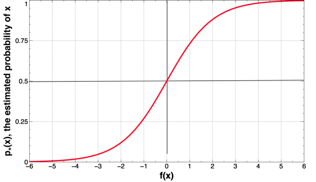
Figure 4-10 plots the estimated probability (vertical axis) as a function of the distance from the decision boundary (horizontal axis). The figure shows that at the decision boundary (at distance x = 0), the probability is 0.5 (a coin toss). The probability varies approximately linearly near to the decision boundary, but then approaches certainty farther away. Part of the “fitting” of the model to the data includes determining the slope of the almost-linear part, and thereby how quickly we are certain of the class as we move away from the boundary.

The other main technical point that we omitted in our main discussion above is: what then is the objective function we use to fit the logistic regression model to the data? Recall that the training data have binary values of the target variable. The model can be applied to the training data to produce estimates that each of the training data points belongs to the target class. What would we want? Ideally, any positive example x₊ would have and any negative example x_• would have . Unfortunately, with real-world data it is unlikely that we will be able to estimate these probabilities perfectly (consider the task of estimating that a consumer described by demographic variables would respond to a particular offer). Nevertheless, we still would like to be as close as possible to one and to be as close as possible to zero.

This leads us to the standard objective function for fitting a logistic regression model to data. Consider the following function computing the “likelihood” that a particular labeled example belongs to the correct class, given a set of parameters w that produces class probability estimates :

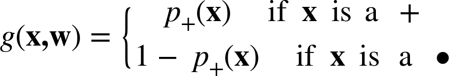
The g function gives the model’s estimated probability of seeing x’s actual class given x’s features. Now consider summing the g values across all the examples in a labeled dataset. And do that for different parameterized models—in our case, different sets of weights (w) for the logistic regression. The model (set of weights) that gives the highest sum is the model that gives the highest “likelihood” to the data—the “maximum likelihood” model. The maximum likelihood model “on average” gives the highest probabilities to the positive examples and the lowest probabilities to the negative examples.

Class Labels and Probabilities

One may be tempted to think that the target variable is a representation of the probability of class membership, and the observed values of the target variable in the training data simply report probabilities of p(x) = 1 for cases that are observed to be in the class and p(x) = 0 for instances that are observed not to be in the class. However, this is not generally consistent with how logistic regression models are used. Take an application to targeted marketing for example. For a consumer c, our model may estimate the probability of responding to the offer to be . In the data, we see that the person indeed does respond. That does not mean that this consumer’s probability of responding actually was 1.0, nor that the model incurred a large error on this example. The consumer’s probability may indeed have been around p(c responds) = 0.02, which actually is a high probability of response for many campaigns, and the consumer just happened to respond this time.

A more satisfying way to think about it is that the training data comprise a set of statistical “draws” from the underlying probabilities, rather than representing the underlying probabilities themselves. The logistic regression procedure then tries to estimate the probabilities (the probability distribution over the instance space) with a linear-log-odds model, based on the observed data on the result of the draws from the distribution.

Example: Logistic Regression versus Tree Induction

Though classification trees and linear classifiers both use linear decision boundaries, there are two important differences between them:

1. A classification tree uses decision boundaries that are perpendicular to the instance-space axes (see Figure 4-1), whereas the linear classifier can use decision boundaries of any direction or orientation (see Figure 4-3). This is a direct consequence of the fact that classification trees select a single attribute at a time whereas linear classifiers use a weighted combination of all attributes.
2. A classification tree is a “piecewise” classifier that segments the instance space recursively when it has to, using a divide-and-conquer approach. In principle, a classification tree can cut up the instance space arbitrarily finely into very small regions (though we will see reasons to avoid that in Chapter 5). A linear classifier places a single decision surface through the entire space. It has great freedom in the orientation of the surface, but it is limited to a single division into two segments. This is a direct consequence of there being a single (linear) equation that uses all of the variables, and must fit the entire data space.

It is usually not easy to determine in advance which of these characteristics are a better match to a given dataset. You likely will not know what the best decision boundary will look like. So practically speaking, what are the consequences of these differences?

When applied to a business problem, there is a difference in the comprehensibility of the models to stakeholders with different backgrounds. For example, what exactly a logistic regression model is doing can be quite understandable to people with a strong background in statistics, and very difficult to understand for those who do not. A decision tree, if it is not too large, may be considerably more understandable to someone without a strong statistics or mathematics background.

Why is this important? For many business problems, the data science team does not have the ultimate say in which models are used or implemented. Often there is at least one manager who must “sign off” on the use of a model in practice, and in many cases a set of stakeholders need to be satisfied with the model. For example, to put in place a new model to dispatch technicians to repair problems after customer calls to the telephone company, managers from operations support, customer service, and technical development all need to be satisfied that the new model will do more good than harm—since for this problem no model is perfect.

Let’s try logistic regression on a simple but realistic dataset, the Wisconsin Breast Cancer Dataset. As with the Iris data set from a few sections back and the Mushroom dataset from the previous chapter, this is another popular dataset from the the machine learning dataset repository at the University of California at Irvine.

Each example describes characteristics of a cell nuclei image, which has been labeled as either benign or malignant (cancerous), based on an expert’s diagnosis of the cells. A sample cell image is shown in Figure 4-11.

Figure 4-11. One of the cell images from which the Wisconsin Breast Cancer dataset was derived. (Image courtesy of Nick Street and Bill Wolberg.)

From each image 10 fundamental characteristics were extracted, listed in Table 4-3.

Table 4-3. The attributes of the Wisconsin Breast Cancer dataset.

Attribute name	Description
RADIUS	Mean of distances from center to points on the perimeter
TEXTURE	Standard deviation of grayscale values
PERIMETER	Perimeter of the mass
AREA	Area of the mass
SMOOTHNESS	Local variation in radius lengths
COMPACTNESS	Computed as: perimeter2/area – 1.0
CONCAVITY	Severity of concave portions of the contour
CONCAVE POINTS	Number of concave portions of the contour
SYMMETRY	A measure of the symmetry of the nuclei
FRACTAL DIMENSION	'Coastline approximation' – 1.0
DIAGNOSIS (Target)	Diagnosis of cell sample: malignant or benign

These were “computed from a digitized image of a fine needle aspirate (FNA) of a breast mass. They describe characteristics of the cell nuclei present in the image.” From each of these basic characteristics, three values were computed: the mean (_mean), standard error (_SE), and “worst” or largest (mean of the three largest values, _worst). This resulted in 30 measured attributes in the dataset. There are 357 benign images and 212 malignant images.

Table 4-4. Linear equation learned by logistic regression on the Wisconsin Breast Cancer dataset (see text and Table 4-3 for a description of the attributes).

Attribute	Weight (learned parameter)
SMOOTHNESS_worst	22.3
CONCAVE_mean	19.47
CONCAVE_worst	11.68
SYMMETRY_worst	4.99
CONCAVITY_worst	2.86
CONCAVITY_mean	2.34
RADIUS_worst	0.25
TEXTURE_worst	0.13
AREA_SE	0.06
TEXTURE_mean	0.03
TEXTURE_SE	–0.29
COMPACTNESS_mean	–7.1
COMPACTNESS_SE	–27.87
w0 (intercept)	–17.7

Table 4-4 shows the linear model learned by logistic regression to predict benign versus malignant for this dataset. Specifically, it shows the nonzero weights ordered from highest to lowest.

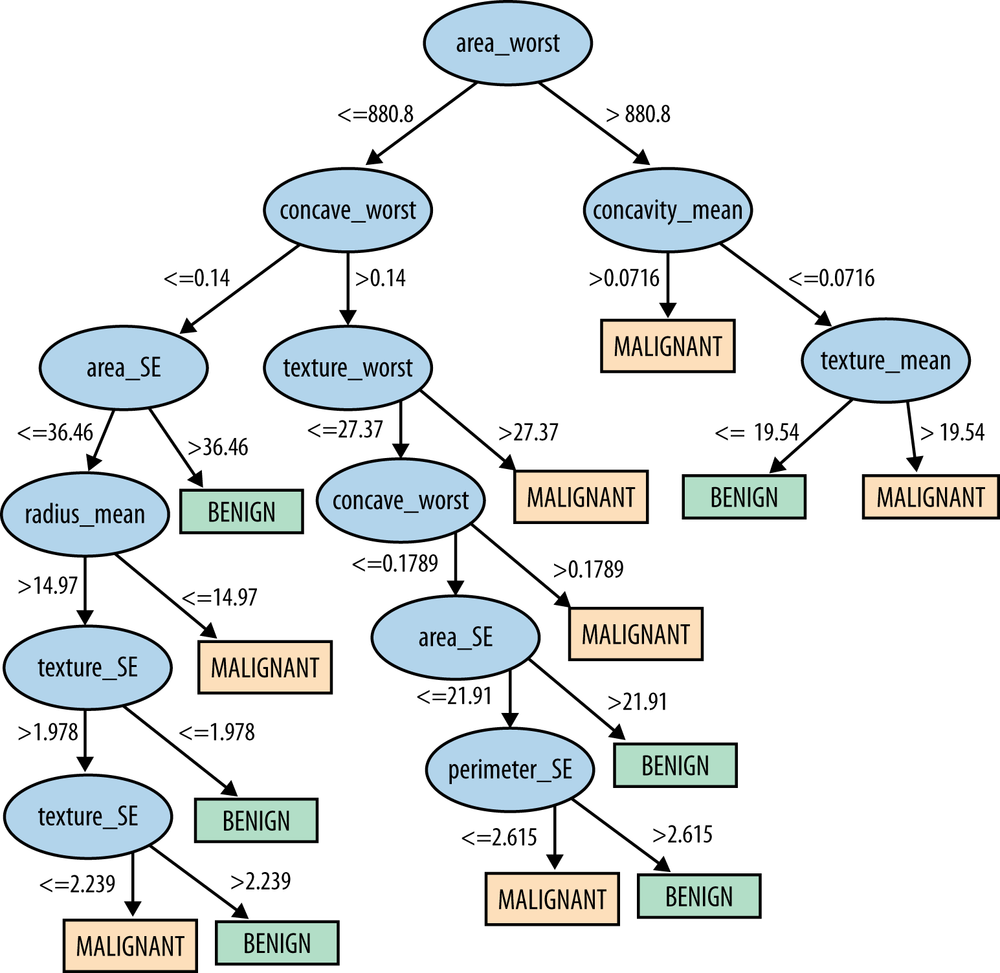
The performance of this model is quite good—it makes only six mistakes on the entire dataset, yielding an accuracy of about 98.9% (the percentage of the instances that the model classifies correctly). For comparison, a classification tree was learned from the same dataset (using Weka’s J48 implementation). The resulting tree is shown in Figure 4-12. The tree has 25 nodes altogether, with 13 leaf nodes. Recall that this means that the tree model partitions the instances into 13 segments. The classification tree’s accuracy is 99.1%, slightly higher than that of logistic regression.

Figure 4-12. Decision tree learned from the Wisconsin Breast Cancer dataset.

The intent of this experiment is only to illustrate the results of two different methods on a dataset, but it is worth digressing briefly to think about these performance results. First, an accuracy figure like 98.9% sounds like a very good result. Is it? We see many such accuracy numbers thrown around in the data mining literature, but evaluating classifiers on real-world problems like cancer diagnosis is often difficult and complex. We discuss evaluation in detail in Chapter 7 and Chapter 8.

Second, consider the two performance results here: 98.9% versus 99.1%. Since the classification tree gives slightly higher accuracy, we might be tempted to conclude that it’s the better model. Should we believe this? This difference is caused by only a single additional error out of the 569 examples. Furthermore, the accuracy numbers were derived by evaluating each model on the same set of examples it was built from. How confident should we be in this evaluation? Chapter 5, Chapter 7, and Chapter 8 discuss guidelines and pitfalls of model evaluation.

Nonlinear Functions, Support Vector Machines, and Neural Networks

So far this chapter has focused on the numeric functions most commonly used in data science: linear models. This set of models includes a wide variety of different techniques. In addition, in Figure 4-13 we show that such linear functions can actually represent nonlinear models, if we include more complex features in the functions. In this example, we used the Iris dataset from An Example of Mining a Linear Discriminant from Data and added a squared term to the input data: Sepal width². The resulting model is a curved line (a parabola) in the original feature space. We also added a single data point to the original dataset, an Iris Versicolor example added at (4, 0.7), shown starred.

Our fundamental concept is much more general than just the application of fitting linear functions. Of course, we could specify arbitrarily complex numeric functions and fit their parameters to the data. The two most common families of techniques that are based on fitting the parameters of complex, nonlinear functions are nonlinear support-vector machines and neural networks.

Figure 4-13. The Iris dataset with a nonlinear feature. In this figure, logistic regression and support vector machine—both linear models—are provided an additional feature, Sepal width², which allows both the freedom to create more complex, nonlinear models (boundaries), as shown.

One can think of nonlinear support vector machines as essentially a systematic way of implementing the “trick” we just discussed of adding more complex terms and fitting a linear function to them. Support vector machines have a so-called “kernel function” that maps the original features to some other feature space. Then a linear model is fit to this new feature space, just as in our simple example in Figure 4-13. Generalizing this, one could implement a nonlinear support vector machine with a “polynomial kernel,” which essentially means it would consider “higher-order” combinations of the original features (e.g., squared features, products of features). A data scientist would become familiar with the different alternatives for kernel functions (linear, polynomial, and others).

Neural networks also implement complex nonlinear numeric functions, based on the fundamental concepts of this chapter. Neural networks offer an intriguing twist. One can think of a neural network as a “stack” of models. On the bottom of the stack are the original features. From these features are learned a variety of relatively simple models. Let’s say these are logistic regressions. Then, each subsequent layer in the stack applies a simple model (let’s say, another logistic regression) to the outputs of the next layer down. So in a two-layer stack, we would learn a set of logistic regressions from the original features, and then learn a logistic regression using as features the outputs of the first set of logistic regressions. We could think of this very roughly as first creating a set of “experts” in different facets of the problem (the first-layer models), and then learning how to weight the opinions of these different experts (the second-layer model).^[27]

The idea of neural networks gets even more intriguing. We might ask: if we are learning those lower-layer logistic regressions—the different experts—what would be the target variable for each? While some practitioners build stacked models where the lower-layer experts are built to represent specific things using specific target variables (e.g., Perlich et al., 2013), more generally with neural networks target labels for training are provided only for the final layer (the actual target variable). So how are the lower-layer logistic regressions trained? We can understand by returning to the fundamental concept of this chapter. The stack of models can be represented by one big parameterized numeric function. The parameters now are the coefficients of all the models, taken together. So once we have decided on an objective function representing what we want to optimize (e.g., the fit to the training data, based on some fitting function), we can then apply an optimization procedure to find the best parameters to this very complex numeric function. When we’re done, we have the parameters to all the models, and thereby have learned the “best” set of lower-level experts and also the best way to combine them, all simultaneously.

Note: Neural networks are useful for many tasks

This section describes neural networks for classification and regression. The field of neural networks is broad and deep, with a long history. Neural networks have found wide application throughout data mining. They are commonly used for many other tasks mentioned in Chapter 2, such as clustering, time series analysis, profiling, and so on.

So, given how cool that sounds, why wouldn’t we want to do that all the time? The tradeoff is that as we increase the amount of flexibility we have to fit the data, we increase the chance that we fit the data too well. The model can fit details of its particular training set rather than finding patterns or models that apply more generally. Specifically, we really want models that apply to other data drawn from the same population or application. This concern is not specific to neural networks, but is very general. It is one of the most important concepts in data science—and it is the subject of the next chapter.

Summary

This chapter introduced a second type of predictive modeling technique called function fitting or parametric modeling. In this case the model is a partially specified equation: a numeric function of the data attributes, with some unspecified numeric parameters. The task of the data mining procedure is to “fit” the model to the data by finding the best set of parameters, in some sense of “best.”

There are many varieties of function fitting techniques, but most use the same linear model structure: a simple weighted sum of the attribute values. The parameters to be fit by the data mining are the weights on the attributes. Linear modeling techniques include traditional linear regression, logistic regression, and linear discriminants such as support-vector machines. Conceptually the key difference between these techniques is their answer to a key issue, What exactly do we mean by best fitting the data? The goodness of fit is described by an “objective function,” and each technique uses a different function. The resulting techniques may be quite different.

We now have seen two very different sorts of data modeling, tree induction and function fitting, and have compared them (in Example: Logistic Regression versus Tree Induction). We have also introduced two criteria by which models can be evaluated: the predictive performance of a model and its intelligibility. It is often advantageous to build different sorts of models from a dataset to gain insight.

This chapter focused on the fundamental concept of optimizing a model’s fit to data. However, doing this leads to the most important fundamental problem with data mining—if you look hard enough, you will find structure in a dataset, even if it’s just there by chance. This tendency is known as overfitting. Recognizing and avoiding overfitting is an important general topic in data science; and we devote the entire next chapter to it.

---

^[21] In order that the line need not go through the origin, it is typical to include the weight w₀, which is the intercept.

^[22] And sometimes it can be surprisingly hard for them to admit it.

^[23] We added the starred point to the original dataset to emphasize the difference in the discriminating lines produced by the two procedures.

^[24] There is an immense literature on linear regression for descriptive analysis of data, and we encourage the reader to delve into it. In this book, we treat linear regression simply as one of many modeling techniques. Our treatment does differ from what you are likely to have learned about regression analysis, because we focus on linear regression for making predictions. Other authors have discussed in detail the differences between descriptive modeling and predictive modeling (Shmueli, 2010).

^[25] Gauss agreed with objections to the arbitrariness of this choice.

^[26] Often technical treatments use the “hat” notation, p̂, to differentiate the model’s estimate of the probability of class membership from the actual probability of class membership. We will not use the hat, but the technically savvy reader should keep that in mind.

^[27] Compare this with the notion of ensemble methods described in Chapter 12.