Database Internals

Chapter 1. Introduction and Overview

Database management systems can serve different purposes: some are used primarily for temporary hot data, some serve as a long-lived cold storage, some allow complex analytical queries, some only allow accessing values by the key, some are optimized to store time-series data, and some store large blobs efficiently. To understand differences and draw distinctions, we start with a short classification and overview, as this helps us to understand the scope of further discussions.

Terminology can sometimes be ambiguous and hard to understand without a complete context. For example, distinctions between column and wide column stores that have little or nothing to do with each other, or how clustered and nonclustered indexes relate to index-organized tables. This chapter aims to disambiguate these terms and find their precise definitions.

We start with an overview of database management system architecture (see “DBMS Architecture”), and discuss system components and their responsibilities. After that, we discuss the distinctions among the database management systems in terms of a storage medium (see “Memory- Versus Disk-Based DBMS”), and layout (see “Column- Versus Row-Oriented DBMS”).

These two groups do not present a full taxonomy of database management systems and there are many other ways they’re classified. For example, some sources group DBMSs into three major categories:

Online transaction processing (OLTP) databases

These handle a large number of user-facing requests and transactions. Queries are often predefined and short-lived.

Online analytical processing (OLAP) databases

These handle complex aggregations. OLAP databases are often used for analytics and data warehousing, and are capable of handling complex, long-running ad hoc queries.

Hybrid transactional and analytical processing (HTAP)

These databases combine properties of both OLTP and OLAP stores.

There are many other terms and classifications: key-value stores, relational databases, document-oriented stores, and graph databases. These concepts are not defined here, since the reader is assumed to have a high-level knowledge and understanding of their functionality. Because the concepts we discuss here are widely applicable and are used in most of the mentioned types of stores in some capacity, complete taxonomy is not necessary or important for further discussion.

Since Part I of this book focuses on the storage and indexing structures, we need to understand the high-level data organization approaches, and the relationship between the data and index files (see “Data Files and Index Files”).

Finally, in “Buffering, Immutability, and Ordering”, we discuss three techniques widely used to develop efficient storage structures and how applying these techniques influences their design and implementation.

DBMS Architecture

There’s no common blueprint for database management system design. Every database is built slightly differently, and component boundaries are somewhat hard to see and define. Even if these boundaries exist on paper (e.g., in project documentation), in code seemingly independent components may be coupled because of performance optimizations, handling edge cases, or architectural decisions.

Sources that describe database management system architecture (for example, [HELLERSTEIN07], [WEIKUM01], [ELMASRI11], and [GARCIAMOLINA08]), define components and relationships between them differently. The architecture presented in Figure 1-1 demonstrates some of the common themes in these representations.

Database management systems use a client/server model, where database system instances (nodes) take the role of servers, and application instances take the role of clients.

Client requests arrive through the transport subsystem. Requests come in the form of queries, most often expressed in some query language. The transport subsystem is also responsible for communication with other nodes in the database cluster.

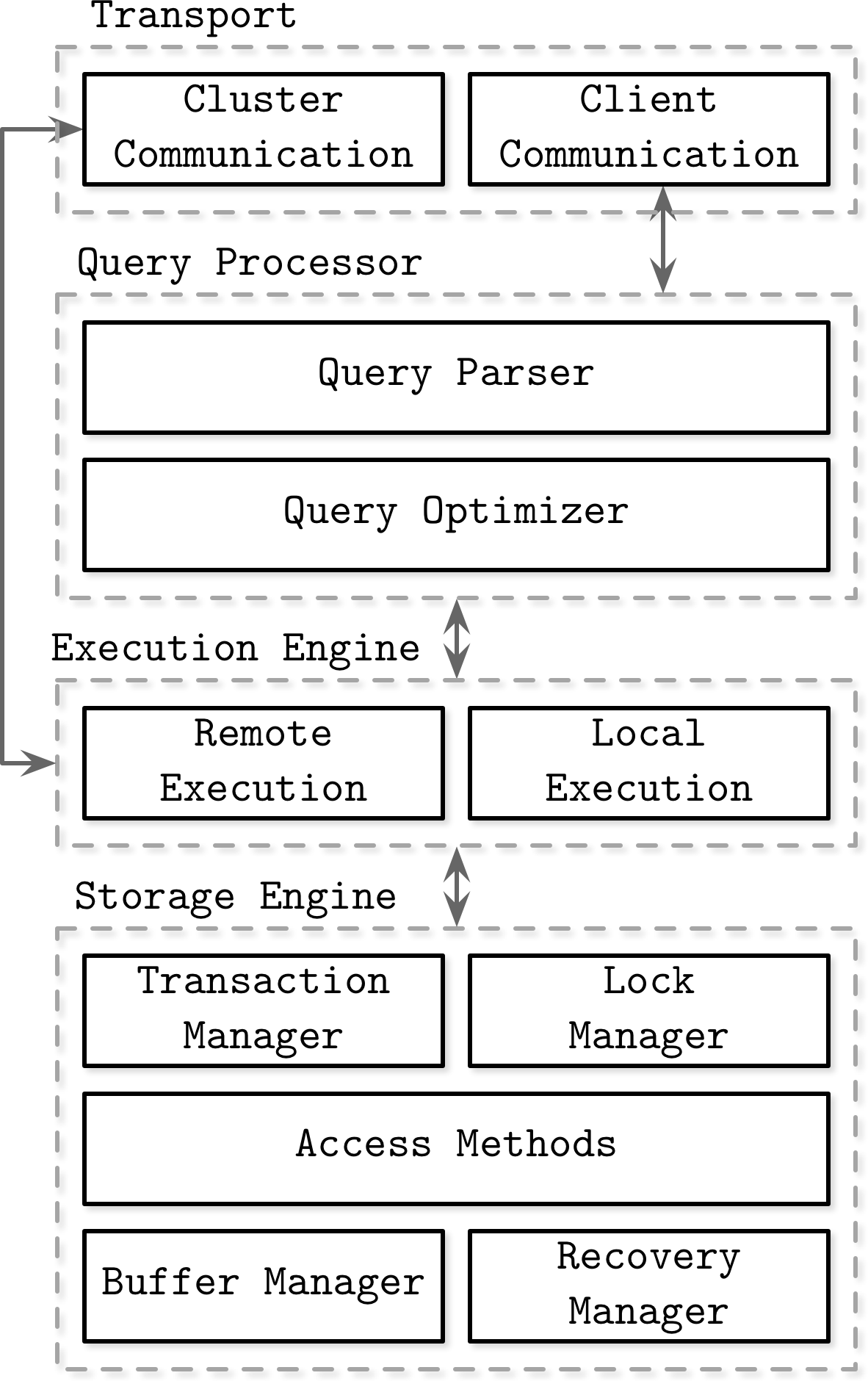
Figure 1-1. Architecture of a database management system

Upon receipt, the transport subsystem hands the query over to a query processor, which parses, interprets, and validates it. Later, access control checks are performed, as they can be done fully only after the query is interpreted.

The parsed query is passed to the query optimizer, which first eliminates impossible and redundant parts of the query, and then attempts to find the most efficient way to execute it based on internal statistics (index cardinality, approximate intersection size, etc.) and data placement (which nodes in the cluster hold the data and the costs associated with its transfer). The optimizer handles both relational operations required for query resolution, usually presented as a dependency tree, and optimizations, such as index ordering, cardinality estimation, and choosing access methods.

The query is usually presented in the form of an execution plan (or query plan): a sequence of operations that have to be carried out for its results to be considered complete. Since the same query can be satisfied using different execution plans that can vary in efficiency, the optimizer picks the best available plan.

The execution plan is carried out by the execution engine, which aggregates the results of local and remote operations. Remote execution can involve writing and reading data to and from other nodes in the cluster, and replication.

Local queries (coming directly from clients or from other nodes) are executed by the storage engine. The storage engine has several components with dedicated responsibilities:

Transaction manager

This manager schedules transactions and ensures they cannot leave the database in a logically inconsistent state.

Lock manager

This manager locks on the database objects for the running transactions, ensuring that concurrent operations do not violate physical data integrity.

Access methods (storage structures)

These manage access and organizing data on disk. Access methods include heap files and storage structures such as B-Trees (see “Ubiquitous B-Trees”) or LSM Trees (see “LSM Trees”).

Buffer manager

This manager caches data pages in memory (see “Buffer Management”).

Recovery manager

This manager maintains the operation log and restoring the system state in case of a failure (see “Recovery”).

Together, transaction and lock managers are responsible for concurrency control (see “Concurrency Control”): they guarantee logical and physical data integrity while ensuring that concurrent operations are executed as efficiently as possible.

Memory- Versus Disk-Based DBMS

Database systems store data in memory and on disk. In-memory database management systems (sometimes called main memory DBMS) store data primarily in memory and use the disk for recovery and logging. Disk-based DBMS hold most of the data on disk and use memory for caching disk contents or as a temporary storage. Both types of systems use the disk to a certain extent, but main memory databases store their contents almost exclusively in RAM.

Accessing memory has been and remains several orders of magnitude faster than accessing disk,¹ so it is compelling to use memory as the primary storage, and it becomes more economically feasible to do so as memory prices go down. However, RAM prices still remain high compared to persistent storage devices such as SSDs and HDDs.

Main memory database systems are different from their disk-based counterparts not only in terms of a primary storage medium, but also in which data structures, organization, and optimization techniques they use.

Databases using memory as a primary data store do this mainly because of performance, comparatively low access costs, and access granularity. Programming for main memory is also significantly simpler than doing so for the disk. Operating systems abstract memory management and allow us to think in terms of allocating and freeing arbitrarily sized memory chunks. On disk, we have to manage data references, serialization formats, freed memory, and fragmentation manually.

The main limiting factors on the growth of in-memory databases are RAM volatility (in other words, lack of durability) and costs. Since RAM contents are not persistent, software errors, crashes, hardware failures, and power outages can result in data loss. There are ways to ensure durability, such as uninterrupted power supplies and battery-backed RAM, but they require additional hardware resources and operational expertise. In practice, it all comes down to the fact that disks are easier to maintain and have significantly lower prices.

The situation is likely to change as the availability and popularity of Non-Volatile Memory (NVM) [ARULRAJ17] technologies grow. NVM storage reduces or completely eliminates (depending on the exact technology) asymmetry between read and write latencies, further improves read and write performance, and allows byte-addressable access.

Durability in Memory-Based Stores

In-memory database systems maintain backups on disk to provide durability and prevent loss of the volatile data. Some databases store data exclusively in memory, without any durability guarantees, but we do not discuss them in the scope of this book.

Before the operation can be considered complete, its results have to be written to a sequential log file. We discuss write-ahead logs in more detail in “Recovery”. To avoid replaying complete log contents during startup or after a crash, in-memory stores maintain a backup copy. The backup copy is maintained as a sorted disk-based structure, and modifications to this structure are often asynchronous (decoupled from client requests) and applied in batches to reduce the number of I/O operations. During recovery, database contents can be restored from the backup and logs.

Log records are usually applied to backup in batches. After the batch of log records is processed, backup holds a database snapshot for a specific point in time, and log contents up to this point can be discarded. This process is called checkpointing. It reduces recovery times by keeping the disk-resident database most up-to-date with log entries without requiring clients to block until the backup is updated.

Note

It is unfair to say that the in-memory database is the equivalent of an on-disk database with a huge page cache (see “Buffer Management”). Even though pages are cached in memory, serialization format and data layout incur additional overhead and do not permit the same degree of optimization that in-memory stores can achieve.

Disk-based databases use specialized storage structures, optimized for disk access. In memory, pointers can be followed comparatively quickly, and random memory access is significantly faster than the random disk access. Disk-based storage structures often have a form of wide and short trees (see “Trees for Disk-Based Storage”), while memory-based implementations can choose from a larger pool of data structures and perform optimizations that would otherwise be impossible or difficult to implement on disk [GARCIAMOLINA92]. Similarly, handling variable-size data on disk requires special attention, while in memory it’s often a matter of referencing the value with a pointer.

For some use cases, it is reasonable to assume that an entire dataset is going to fit in memory. Some datasets are bounded by their real-world representations, such as student records for schools, customer records for corporations, or inventory in an online store. Each record takes up not more than a few Kb, and their number is limited.

Column- Versus Row-Oriented DBMS

Most database systems store a set of data records, consisting of columns and rows in tables. Field is an intersection of a column and a row: a single value of some type. Fields belonging to the same column usually have the same data type. For example, if we define a table holding user records, all names would be of the same type and belong to the same column. A collection of values that belong logically to the same record (usually identified by the key) constitutes a row.

One of the ways to classify databases is by how the data is stored on disk: row- or column-wise. Tables can be partitioned either horizontally (storing values belonging to the same row together), or vertically (storing values belonging to the same column together). Figure 1-2 depicts this distinction: (a) shows the values partitioned column-wise, and (b) shows the values partitioned row-wise.

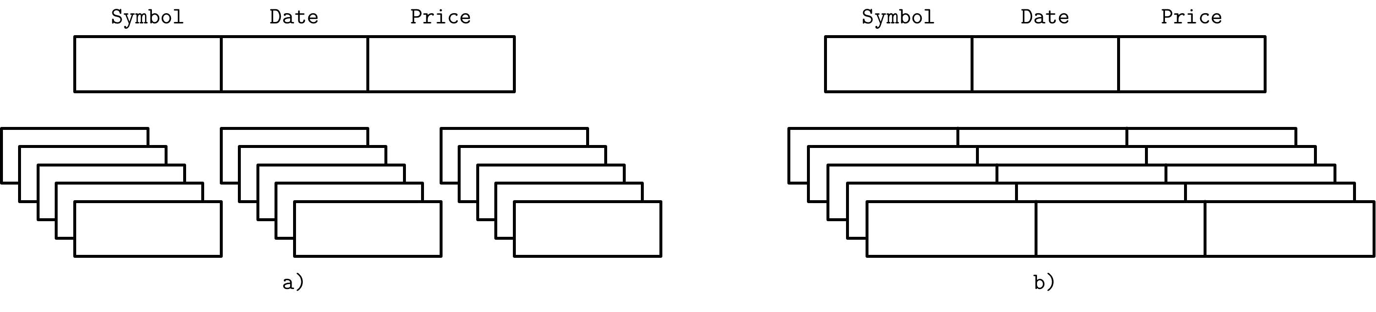
Figure 1-2. Data layout in column- and row-oriented stores

Examples of row-oriented database management systems are abundant: MySQL, PostgreSQL, and most of the traditional relational databases. The two pioneer open source column-oriented stores are MonetDB and C-Store (C-Store is an open source predecessor to Vertica).

Row-Oriented Data Layout

Row-oriented database management systems store data in records or rows. Their layout is quite close to the tabular data representation, where every row has the same set of fields. For example, a row-oriented database can efficiently store user entries, holding names, birth dates, and phone numbers:

| ID | Name  | Birth Date  | Phone Number   |
| 10 | John  | 01 Aug 1981 | [phone] |
| 20 | Sam   | 14 Sep 1988 | [phone] |
| 30 | Keith | 07 Jan 1984 | [phone] |

This approach works well for cases where several fields constitute the record (name, birth date, and a phone number) uniquely identified by the key (in this example, a monotonically incremented number). All fields representing a single user record are often read together. When creating records (for example, when the user fills out a registration form), we write them together as well. At the same time, each field can be modified individually.

Since row-oriented stores are most useful in scenarios when we have to access data by row, storing entire rows together improves spatial locality² [DENNING68].

Because data on a persistent medium such as a disk is typically accessed block-wise (in other words, a minimal unit of disk access is a block), a single block will contain data for all columns. This is great for cases when we’d like to access an entire user record, but makes queries accessing individual fields of multiple user records (for example, queries fetching only the phone numbers) more expensive, since data for the other fields will be paged in as well.

Column-Oriented Data Layout

Column-oriented database management systems partition data vertically (i.e., by column) instead of storing it in rows. Here, values for the same column are stored contiguously on disk (as opposed to storing rows contiguously as in the previous example). For example, if we store historical stock market prices, price quotes are stored together. Storing values for different columns in separate files or file segments allows efficient queries by column, since they can be read in one pass rather than consuming entire rows and discarding data for columns that weren’t queried.

Column-oriented stores are a good fit for analytical workloads that compute aggregates, such as finding trends, computing average values, etc. Processing complex aggregates can be used in cases when logical records have multiple fields, but some of them (in this case, price quotes) have different importance and are often consumed together.

From a logical perspective, the data representing stock market price quotes can still be expressed as a table:

| ID | Symbol | Date        | Price     |
| 1  | DOW    | 08 Aug 2018 | 24,314.65 |
| 2  | DOW    | 09 Aug 2018 | 24,136.16 |
| 3  | S&P    | 08 Aug 2018 | 2,414.45  |
| 4  | S&P    | 09 Aug 2018 | 2,232.32  |

However, the physical column-based database layout looks entirely different. Values belonging to the same column are stored closely together:

Symbol: 1:DOW; 2:DOW; 3:S&P; 4:S&P
Date:   1:08 Aug 2018; 2:09 Aug 2018; 3:08 Aug 2018; 4:09 Aug 2018
Price:  1:24,314.65; 2:24,136.16; 3:2,414.45; 4:2,232.32

To reconstruct data tuples, which might be useful for joins, filtering, and multirow aggregates, we need to preserve some metadata on the column level to identify which data points from other columns it is associated with. If you do this explicitly, each value will have to hold a key, which introduces duplication and increases the amount of stored data. Some column stores use implicit identifiers (virtual IDs) instead and use the position of the value (in other words, its offset) to map it back to the related values [ABADI13].

During the last several years, likely due to a rising demand to run complex analytical queries over growing datasets, we’ve seen many new column-oriented file formats such as Apache Parquet, Apache ORC, RCFile, as well as column-oriented stores, such as Apache Kudu, ClickHouse, and many others [ROY12].

Distinctions and Optimizations

It is not sufficient to say that distinctions between row and column stores are only in the way the data is stored. Choosing the data layout is just one of the steps in a series of possible optimizations that columnar stores are targeting.

Reading multiple values for the same column in one run significantly improves cache utilization and computational efficiency. On modern CPUs, vectorized instructions can be used to process multiple data points with a single CPU instruction³ [DREPPER07].

Storing values that have the same data type together (e.g., numbers with other numbers, strings with other strings) offers a better compression ratio. We can use different compression algorithms depending on the data type and pick the most effective compression method for each case.

To decide whether to use a column- or a row-oriented store, you need to understand your access patterns. If the read data is consumed in records (i.e., most or all of the columns are requested) and the workload consists mostly of point queries and range scans, the row-oriented approach is likely to yield better results. If scans span many rows, or compute aggregate over a subset of columns, it is worth considering a column-oriented approach.

Wide Column Stores

Column-oriented databases should not be mixed up with wide column stores, such as BigTable or HBase, where data is represented as a multidimensional map, columns are grouped into column families (usually storing data of the same type), and inside each column family, data is stored row-wise. This layout is best for storing data retrieved by a key or a sequence of keys.

A canonical example from the Bigtable paper [CHANG06] is a Webtable. A Webtable stores snapshots of web page contents, their attributes, and the relations among them at a specific timestamp. Pages are identified by the reversed URL, and all attributes (such as page content and anchors, representing links between pages) are identified by the timestamps at which these snapshots were taken. In a simplified way, it can be represented as a nested map, as Figure 1-3 shows.

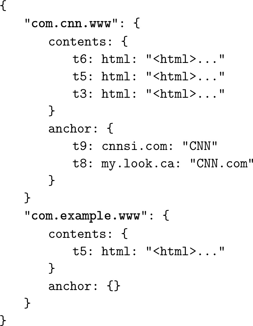
Figure 1-3. Conceptual structure of a Webtable

Data is stored in a multidimensional sorted map with hierarchical indexes: we can locate the data related to a specific web page by its reversed URL and its contents or anchors by the timestamp. Each row is indexed by its row key. Related columns are grouped together in column families—contents and anchor in this example—which are stored on disk separately. Each column inside a column family is identified by the column key, which is a combination of the column family name and a qualifier (html, cnnsi.com, my.look.ca in this example). Column families store multiple versions of data by timestamp. This layout allows us to quickly locate the higher-level entries (web pages, in this case) and their parameters (versions of content and links to the other pages).

While it is useful to understand the conceptual representation of wide column stores, their physical layout is somewhat different. A schematic representation of the data layout in column families is shown in Figure 1-4: column families are stored separately, but in each column family, the data belonging to the same key is stored together.

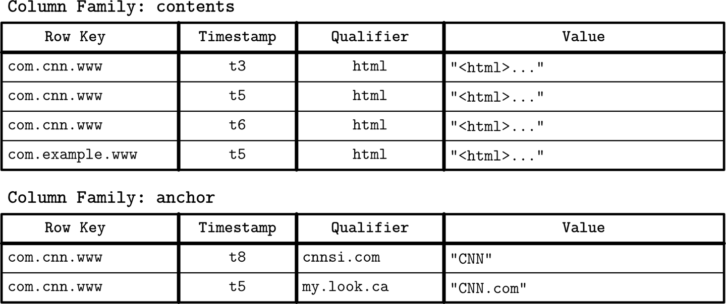
Figure 1-4. Physical structure of a Webtable

Data Files and Index Files

The primary goal of a database system is to store data and to allow quick access to it. But how is the data organized? Why do we need a database management system and not just a bunch of files? How does file organization improve efficiency?

Database systems do use files for storing the data, but instead of relying on filesystem hierarchies of directories and files for locating records, they compose files using implementation-specific formats. The main reasons to use specialized file organization over flat files are:

Storage efficiency

Files are organized in a way that minimizes storage overhead per stored data record.

Access efficiency

Records can be located in the smallest possible number of steps.

Update efficiency

Record updates are performed in a way that minimizes the number of changes on disk.

Database systems store data records, consisting of multiple fields, in tables, where each table is usually represented as a separate file. Each record in the table can be looked up using a search key. To locate a record, database systems use indexes: auxiliary data structures that allow it to efficiently locate data records without scanning an entire table on every access. Indexes are built using a subset of fields identifying the record.

A database system usually separates data files and index files: data files store data records, while index files store record metadata and use it to locate records in data files. Index files are typically smaller than the data files. Files are partitioned into pages, which typically have the size of a single or multiple disk blocks. Pages can be organized as sequences of records or as a slotted pages (see “Slotted Pages”).

New records (insertions) and updates to the existing records are represented by key/value pairs. Most modern storage systems do not delete data from pages explicitly. Instead, they use deletion markers (also called tombstones), which contain deletion metadata, such as a key and a timestamp. Space occupied by the records shadowed by their updates or deletion markers is reclaimed during garbage collection, which reads the pages, writes the live (i.e., nonshadowed) records to the new place, and discards the shadowed ones.

Data Files

Data files (sometimes called primary files) can be implemented as index-organized tables (IOT), heap-organized tables (heap files), or hash-organized tables (hashed files).

Records in heap files are not required to follow any particular order, and most of the time they are placed in a write order. This way, no additional work or file reorganization is required when new pages are appended. Heap files require additional index structures, pointing to the locations where data records are stored, to make them searchable.

In hashed files, records are stored in buckets, and the hash value of the key determines which bucket a record belongs to. Records in the bucket can be stored in append order or sorted by key to improve lookup speed.

Index-organized tables (IOTs) store data records in the index itself. Since records are stored in key order, range scans in IOTs can be implemented by sequentially scanning its contents.

Storing data records in the index allows us to reduce the number of disk seeks by at least one, since after traversing the index and locating the searched key, we do not have to address a separate file to find the associated data record.

When records are stored in a separate file, index files hold data entries, uniquely identifying data records and containing enough information to locate them in the data file. For example, we can store file offsets (sometimes called row locators), locations of data records in the data file, or bucket IDs in the case of hash files. In index-organized tables, data entries hold actual data records.

Index Files

An index is a structure that organizes data records on disk in a way that facilitates efficient retrieval operations. Index files are organized as specialized structures that map keys to locations in data files where the records identified by these keys (in the case of heap files) or primary keys (in the case of index-organized tables) are stored.

An index on a primary (data) file is called the primary index. In most cases we can also assume that the primary index is built over a primary key or a set of keys identified as primary. All other indexes are called secondary.

Secondary indexes can point directly to the data record, or simply store its primary key. A pointer to a data record can hold an offset to a heap file or an index-organized table. Multiple secondary indexes can point to the same record, allowing a single data record to be identified by different fields and located through different indexes. While primary index files hold a unique entry per search key, secondary indexes may hold several entries per search key [GARCIAMOLINA08].

If the order of data records follows the search key order, this index is called clustered (also known as clustering). Data records in the clustered case are usually stored in the same file or in a clustered file, where the key order is preserved. If the data is stored in a separate file, and its order does not follow the key order, the index is called nonclustered (sometimes called unclustered).

Figure 1-5 shows the difference between the two approaches:

• a) An index-organized table, where data records are stored directly in the index file.

• b) An index file storing the offsets and a separate file storing data records.

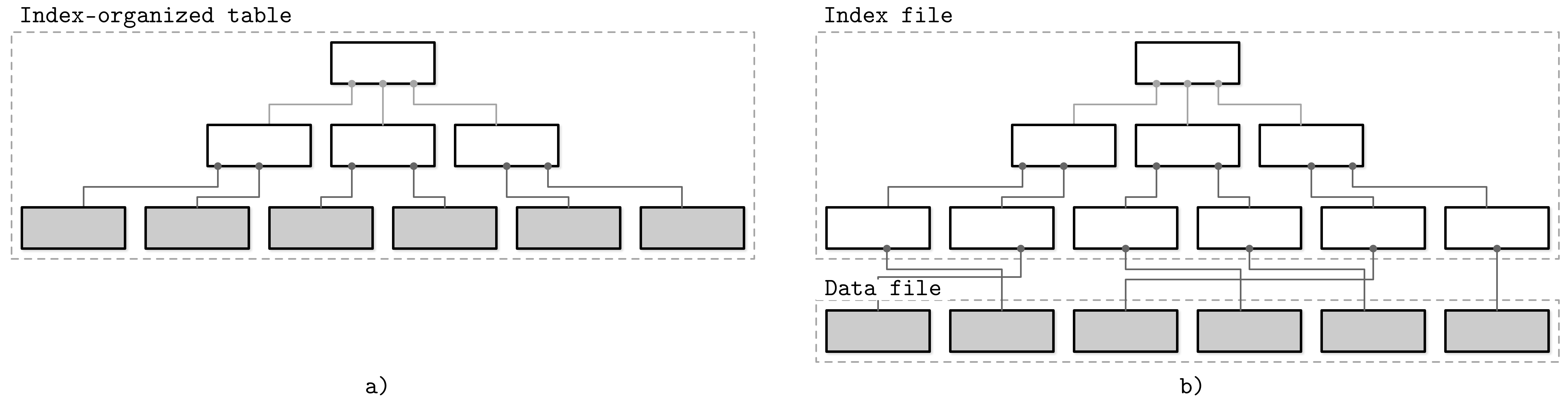
Figure 1-5. Storing data records in an index file versus storing offsets to the data file (index segments shown in white; segments holding data records shown in gray)

Note

Index-organized tables store information in index order and are clustered by definition. Primary indexes are most often clustered. Secondary indexes are nonclustered by definition, since they’re used to facilitate access by keys other than the primary one. Clustered indexes can be both index-organized or have separate index and data files.

Many database systems have an inherent and explicit primary key, a set of columns that uniquely identify the database record. In cases when the primary key is not specified, the storage engine can create an implicit primary key (for example, MySQL InnoDB adds a new auto-increment column and fills in its values automatically).

This terminology is used in different kinds of database systems: relational database systems (such as MySQL and PostgreSQL), Dynamo-based NoSQL stores (such as Apache Cassandra and in Riak), and document stores (such as MongoDB). There can be some project-specific naming, but most often there’s a clear mapping to this terminology.

Primary Index as an Indirection

There are different opinions in the database community on whether data records should be referenced directly (through file offset) or via the primary key index.⁴

Both approaches have their pros and cons and are better discussed in the scope of a complete implementation. By referencing data directly, we can reduce the number of disk seeks, but have to pay a cost of updating the pointers whenever the record is updated or relocated during a maintenance process. Using indirection in the form of a primary index allows us to reduce the cost of pointer updates, but has a higher cost on a read path.

Updating just a couple of indexes might work if the workload mostly consists of reads, but this approach does not work well for write-heavy workloads with multiple indexes. To reduce the costs of pointer updates, instead of payload offsets, some implementations use primary keys for indirection. For example, MySQL InnoDB uses a primary index and performs two lookups: one in the secondary index, and one in a primary index when performing a query [TARIQ11]. This adds an overhead of a primary index lookup instead of following the offset directly from the secondary index.

Figure 1-6 shows how the two approaches are different:

• a) Two indexes reference data entries directly from secondary index files.

• b) A secondary index goes through the indirection layer of a primary index to locate the data entries.

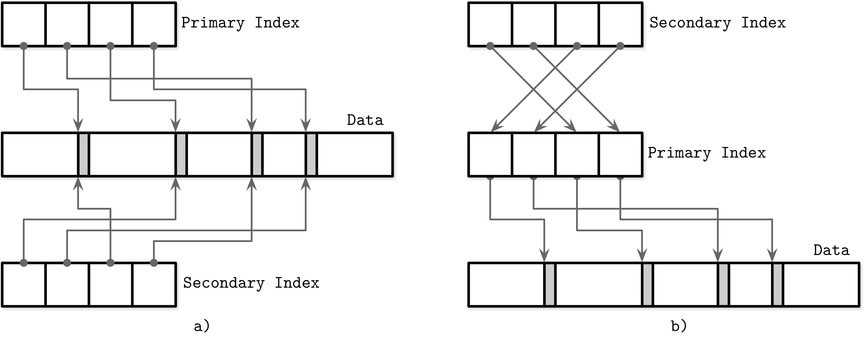
Figure 1-6. Referencing data tuples directly (a) versus using a primary index as indirection (b)

It is also possible to use a hybrid approach and store both data file offsets and primary keys. First, you check if the data offset is still valid and pay the extra cost of going through the primary key index if it has changed, updating the index file after finding a new offset.

Buffering, Immutability, and Ordering

A storage engine is based on some data structure. However, these structures do not describe the semantics of caching, recovery, transactionality, and other things that storage engines add on top of them.

In the next chapters, we will start the discussion with B-Trees (see “Ubiquitous B-Trees”) and try to understand why there are so many B-Tree variants, and why new database storage structures keep emerging.

Storage structures have three common variables: they use buffering (or avoid using it), use immutable (or mutable) files, and store values in order (or out of order). Most of the distinctions and optimizations in storage structures discussed in this book are related to one of these three concepts.

Buffering

This defines whether or not the storage structure chooses to collect a certain amount of data in memory before putting it on disk. Of course, every on-disk structure has to use buffering to some degree, since the smallest unit of data transfer to and from the disk is a block, and it is desirable to write full blocks. Here, we’re talking about avoidable buffering, something storage engine implementers choose to do. One of the first optimizations we discuss in this book is adding in-memory buffers to B-Tree nodes to amortize I/O costs (see “Lazy B-Trees”). However, this is not the only way we can apply buffering. For example, two-component LSM Trees (see “Two-component LSM Tree”), despite their similarities with B-Trees, use buffering in an entirely different way, and combine buffering with immutability.

Mutability (or immutability)

This defines whether or not the storage structure reads parts of the file, updates them, and writes the updated results at the same location in the file. Immutable structures are append-only: once written, file contents are not modified. Instead, modifications are appended to the end of the file. There are other ways to implement immutability. One of them is copy-on-write (see “Copy-on-Write”), where the modified page, holding the updated version of the record, is written to the new location in the file, instead of its original location. Often the distinction between LSM and B-Trees is drawn as immutable against in-place update storage, but there are structures (for example, “Bw-Trees”) that are inspired by B-Trees but are immutable.

Ordering

This is defined as whether or not the data records are stored in the key order in the pages on disk. In other words, the keys that sort closely are stored in contiguous segments on disk. Ordering often defines whether or not we can efficiently scan the range of records, not only locate the individual data records. Storing data out of order (most often, in insertion order) opens up for some write-time optimizations. For example, Bitcask (see “Bitcask”) and WiscKey (see “WiscKey”) store data records directly in append-only files.

Of course, a brief discussion of these three concepts is not enough to show their power, and we’ll continue this discussion throughout the rest of the book.

Summary

In this chapter, we’ve discussed the architecture of a database management system and covered its primary components.

To highlight the importance of disk-based structures and their difference from in-memory ones, we discussed memory- and disk-based stores. We came to the conclusion that disk-based structures are important for both types of stores, but are used for different purposes.

To understand how access patterns influence database system design, we discussed column- and row-oriented database management systems and the primary factors that set them apart from each other. To start a conversation about how the data is stored, we covered data and index files.

Lastly, we introduced three core concepts: buffering, immutability, and ordering. We will use them throughout this book to highlight properties of the storage engines that use them.

Further Reading

If you’d like to learn more about the concepts mentioned in this chapter, you can refer to the following sources:

Database architecture

Hellerstein, Joseph M., Michael Stonebraker, and James Hamilton. 2007. “Architecture of a Database System.” Foundations and Trends in Databases 1, no. 2 (February): 141-259. https://doi.org/10.1561/1900000002.

Column-oriented DBMS

Abadi, Daniel, Peter Boncz, Stavros Harizopoulos, Stratos Idreaos, and Samuel Madden. 2013. The Design and Implementation of Modern Column-Oriented Database Systems. Hanover, MA: Now Publishers Inc.

In-memory DBMS

Faerber, Frans, Alfons Kemper, and Per-Åke Alfons. 2017. Main Memory Database Systems. Hanover, MA: Now Publishers Inc.

¹ You can find a visualization and comparison of disk, memory access latencies, and many other relevant numbers over the years at https://people.eecs.berkeley.edu/~rcs/research/interactive_latency.html.

² Spatial locality is one of the Principles of Locality, stating that if a memory location is accessed, its nearby memory locations will be accessed in the near future.

³ Vectorized instructions, or Single Instruction Multiple Data (SIMD), describes a class of CPU instructions that perform the same operation on multiple data points.

⁴ The original post that has stirred up the discussion was controversial and one-sided, but you can refer to the presentation comparing MySQL and PostgreSQL index and storage formats, which references the original source as well.