Deep Learning from Scratch

Chapter 1. Foundations

Don’t memorize these formulas. If you understand the concepts, you can invent your own notation.

John Cochrane, Investments Notes 2006

The aim of this chapter is to explain some foundational mental models that are essential for understanding how neural networks work. Specifically, we’ll cover nested mathematical functions and their derivatives. We’ll work our way up from the simplest possible building blocks to show that we can build complicated functions made up of a “chain” of constituent functions and, even when one of these functions is a matrix multiplication that takes in multiple inputs, compute the derivative of the functions’ outputs with respect to their inputs. Understanding how this process works will be essential to understanding neural networks, which we technically won’t begin to cover until Chapter 2.

As we’re getting our bearings around these foundational building blocks of neural networks, we’ll systematically describe each concept we introduce from three perspectives:

• Math, in the form of an equation or equations

• Code, with as little extra syntax as possible (making Python an ideal choice)

• A diagram explaining what is going on, of the kind you would draw on a whiteboard during a coding interview

As mentioned in the preface, one of the challenges of understanding neural networks is that it requires multiple mental models. We’ll get a sense of that in this chapter: each of these three perspectives excludes certain essential features of the concepts we’ll cover, and only when taken together do they provide a full picture of both how and why nested mathematical functions work the way they do. In fact, I take the uniquely strong view that any attempt to explain the building blocks of neural networks that excludes one of these three perspectives is incomplete.

With that out of the way, it’s time to take our first steps. We’re going to start with some extremely simple building blocks to illustrate how we can understand different concepts in terms of these three perspectives. Our first building block will be a simple but critical concept: the function.

Functions

What is a function, and how do we describe it? As with neural nets, there are several ways to describe functions, none of which individually paints a complete picture. Rather than trying to give a pithy one-sentence description, let’s simply walk through the three mental models one by one, playing the role of the blind men feeling different parts of the elephant.

Math

Here are two examples of functions, described in mathematical notation:

• f₁(x) = x²

• f₂(x) = max(x, 0)

This notation says that the functions, which we arbitrarily call f₁ and f₂, take in a number x as input and transform it into either x² (in the first case) or max(x, 0) (in the second case).

Diagrams

One way of depicting functions is to:

1. Draw an x-y plane (where x refers to the horizontal axis and y refers to the vertical axis).

2. Plot a bunch of points, where the x-coordinates of the points are (usually evenly spaced) inputs of the function over some range, and the y-coordinates are the outputs of the function over that range.

3. Connect these plotted points.

This was first done by the French philosopher René Descartes, and it is extremely useful in many areas of mathematics, in particular calculus. Figure 1-1 shows the plot of these two functions.

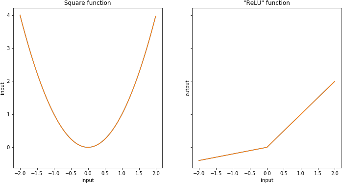
Figure 1-1. Two continuous, mostly differentiable functions

However, there is another way to depict functions that isn’t as useful when learning calculus but that will be very useful for us when thinking about deep learning models. We can think of functions as boxes that take in numbers as input and produce numbers as output, like minifactories that have their own internal rules for what happens to the input. Figure 1-2 shows both these functions described as general rules and how they operate on specific inputs.

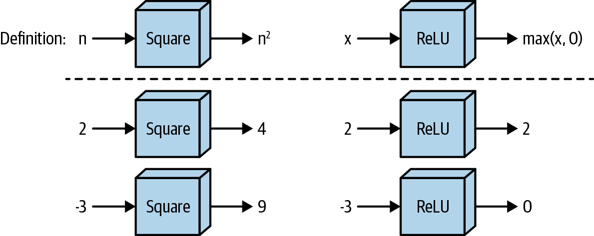
Figure 1-2. Another way of looking at these functions

Code

Finally, we can describe these functions using code. Before we do, we should say a bit about the Python library on top of which we’ll be writing our functions: NumPy.

Code caveat #1: NumPy

NumPy is a widely used Python library for fast numeric computation, the internals of which are mostly written in C. Simply put: the data we deal with in neural networks will always be held in a multidimensional array that is almost always either one-, two-, three-, or four-dimensional, but especially two- or three-dimensional. The ndarray class from the NumPy library allows us to operate on these arrays in ways that are both (a) intuitive and (b) fast. To take the simplest possible example: if we were storing our data in Python lists (or lists of lists), adding or multiplying the lists elementwise using normal syntax wouldn’t work, whereas it does work for ndarrays:

print("Python list operations:")
a = [1,2,3]
b = [4,5,6]
print("a+b:", a+b)
try:
    print(a*b)
except TypeError:
    print("a*b has no meaning for Python lists")
print()
print("numpy array operations:")
a = np.array([1,2,3])
b = np.array([4,5,6])
print("a+b:", a+b)
print("a*b:", a*b)

Python list operations:
a+b: [1, 2, 3, 4, 5, 6]
a*b has no meaning for Python lists

numpy array operations:
a+b: [5 7 9]
a*b: [ 4 10 18]

ndarrays also have several features you’d expect from an n-dimensional array; each ndarray has n axes, indexed from 0, so that the first axis is 0, the second is 1, and so on. In particular, since we deal with 2D ndarrays often, we can think of axis = 0 as the rows and axis = 1 as the columns—see Figure 1-3.

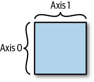
Figure 1-3. A 2D NumPy array, with axis = 0 as the rows and axis = 1 as the columns

NumPy’s ndarrays also support applying functions along these axes in intuitive ways. For example, summing along axis 0 (the rows for a 2D array) essentially “collapses the array” along that axis, returning an array with one less dimension than the original array; for a 2D array, this is equivalent to summing each column:

print('a:')
print(a)
print('a.sum(axis=0):', a.sum(axis=0))
print('a.sum(axis=1):', a.sum(axis=1))

a:
[[1 2]
 [3 4]]
a.sum(axis=0): [4 6]
a.sum(axis=1): [3 7]

Finally, NumPy ndarrays support adding a 1D array to the last axis; for a 2D array a with R rows and C columns, this means we can add a 1D array b of length C and NumPy will do the addition in the intuitive way, adding the elements to each row of a:¹

a = np.array([[1,2,3],
              [4,5,6]])

b = np.array([10,20,30])

print("a+b:\n", a+b)

a+b:
[[11 22 33]
 [14 25 36]]

Code caveat #2: Type-checked functions

As I’ve mentioned, the primary goal of the code we write in this book is to make the concepts I’m explaining precise and clear. This will get more challenging as the book goes on, as we’ll be writing functions with many arguments as part of complicated classes. To combat this, we’ll use functions with type signatures throughout; for example, in Chapter 3, we’ll initialize our neural networks as follows:

def __init__(self,
             layers: List[Layer],
             loss: Loss,
             learning_rate: float = 0.01) -> None:

This type signature alone gives you some idea of what the class is used for. By contrast, consider the following type signature that we could use to define an operation:

def operation(x1, x2):

This type signature by itself gives you no hint as to what is going on; only by printing out each object’s type, seeing what operations get performed on each object, or guessing based on the names x1 and x2 could we understand what is going on in this function. I can instead define a function with a type signature as follows:

def operation(x1: ndarray, x2: ndarray) -> ndarray:

You know right away that this is a function that takes in two ndarrays, probably combines them in some way, and outputs the result of that combination. Because of the increased clarity they provide, we’ll use type-checked functions throughout this book.

Basic functions in NumPy

With these preliminaries in mind, let’s write up the functions we defined earlier in NumPy:

def square(x: ndarray) -> ndarray:
    '''
    Square each element in the input ndarray.
    '''
    return np.power(x, 2)

def leaky_relu(x: ndarray) -> ndarray:
    '''
    Apply "Leaky ReLU" function to each element in ndarray.
    '''
    return np.maximum(0.2 * x, x)

Note

One of NumPy’s quirks is that many functions can be applied to ndarrays either by writing np.function_name(ndarray) or by writing ndarray.function_name. For example, the preceding relu function could be written as: x.clip(min=0). We’ll try to be consistent and use the np.function_name(ndarray) convention throughout—in particular, we’ll avoid tricks such as ndarray.T for transposing a two-dimensional ndarray, instead writing np.transpose(ndarray, (1, 0)).

If you can wrap your mind around the fact that math, a diagram, and code are three different ways of representing the same underlying concept, then you are well on your way to displaying the kind of flexible thinking you’ll need to truly understand deep learning.

Derivatives

Derivatives, like functions, are an extremely important concept for understanding deep learning that many of you are probably familiar with. Also like functions, they can be depicted in multiple ways. We’ll start by simply saying at a high level that the derivative of a function at a point is the “rate of change” of the output of the function with respect to its input at that point. Let’s now walk through the same three perspectives on derivatives that we covered for functions to gain a better mental model for how derivatives work.

Math

First, we’ll get mathematically precise: we can describe this number—how much the output of f changes as we change its input at a particular value a of the input—as a limit:

$$\frac{df}{du}\left(a\right)=\underset{\Delta \to 0}{lim}\frac{f\left(a+\Delta \right)-f\left(a-\Delta \right)}{2\times \Delta }$$

This limit can be approximated numerically by setting a very small value for Δ, such as 0.001, so we can compute the derivative as:

$$\frac{df}{du}\left(a\right)=\frac{f(a+0.001)-f(a-0.001)}{0.002}$$

While accurate, this is only one part of a full mental model of derivatives. Let’s look at them from another perspective: a diagram.

Diagrams

First, the familiar way: if we simply draw a tangent line to the Cartesian representation of the function f, the derivative of f at a point a is just the slope of this line at a. As with the mathematical descriptions in the prior subsection, there are two ways we can actually calculate the slope of this line. The first would be to use calculus to actually calculate the limit. The second would be to just take the slope of the line connecting f at a – 0.001 and a + 0.001. The latter method is depicted in Figure 1-4 and should be familiar to anyone who has taken calculus.

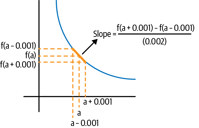
Figure 1-4. Derivatives as slopes

As we saw in the prior section, another way of thinking of functions is as mini-factories. Now think of the inputs to those factories being connected to the outputs by a string. The derivative is equal to the answer to this question: if we pull up on the input to the function a by some very small amount—or, to account for the fact that the function may be asymmetric at a, pull down on a by some small amount—by what multiple of this small amount will the output change, given the inner workings of the factory? This is depicted in Figure 1-5.

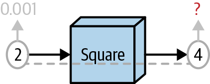
Figure 1-5. Another way of visualizing derivatives

This second representation will turn out to be more important than the first one for understanding deep learning.

Code

Finally, we can code up the approximation to the derivative that we saw previously:

from typing import Callable

def deriv(func: Callable[[ndarray], ndarray],
          input_: ndarray,
          delta: float = 0.001) -> ndarray:
    '''
    Evaluates the derivative of a function "func" at every element in the
    "input_" array.
    '''
    return (func(input_ + delta) - func(input_ - delta)) / (2 * delta)

Note

When we say that “something is a function of something else”—for example, that P is a function of E (letters chosen randomly on purpose), what we mean is that there is some function f such that f(E) = P—or equivalently, there is a function f that takes in E objects and produces P objects. We might also think of this as meaning that P is defined as whatever results when we apply the function f to E:

And we would code this up as:

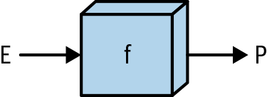
def f(input_: ndarray) -> ndarray:
    # Some transformation(s)
    return output

P = f(E)

Nested Functions

Now we’ll cover a concept that will turn out to be fundamental to understanding neural networks: functions can be “nested” to form “composite” functions. What exactly do I mean by “nested”? I mean that if we have two functions that by mathematical convention we call f₁ and f₂, the output of one of the functions becomes the input to the next one, so that we can “string them together.”

Diagram

The most natural way to represent a nested function is with the “minifactory” or “box” representation (the second representation from “Functions”).

As Figure 1-6 shows, an input goes into the first function, gets transformed, and comes out; then it goes into the second function and gets transformed again, and we get our final output.

Figure 1-6. Nested functions, naturally

Math

We should also include the less intuitive mathematical representation:

$f_2\left(f_1\left(x\right)\right)=y$

This is less intuitive because of the quirk that nested functions are read “from the outside in” but the operations are in fact performed “from the inside out.” For example, though $f_2\left(f_1\left(x\right)\right)=y$ is read “f 2 of f 1 of x,” what it really means is to “first apply f₁ to x, and then apply f₂ to the result of applying f₁ to x.”

Code

Finally, in keeping with my promise to explain every concept from three perspectives, we’ll code this up. First, we’ll define a data type for nested functions:

from typing import List

# A Function takes in an ndarray as an argument and produces an ndarray
Array_Function = Callable[[ndarray], ndarray]

# A Chain is a list of functions
Chain = List[Array_Function]

Then we’ll define how data goes through a chain, first of length 2:

def chain_length_2(chain: Chain,
                   a: ndarray) -> ndarray:
    '''
    Evaluates two functions in a row, in a "Chain".
    '''
    assert len(chain) == 2, \
    "Length of input 'chain' should be 2"

    f1 = chain[0]
    f2 = chain[1]

    return f2(f1(x))

Another Diagram

Depicting the nested function using the box representation shows us that this composite function is really just a single function. Thus, we can represent this function as simply f₁ f₂, as shown in Figure 1-7.

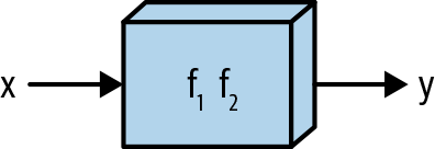
Figure 1-7. Another way to think of nested functions

Moreover, a theorem from calculus tells us that a composite function made up of “mostly differentiable” functions is itself mostly differentiable! Thus, we can think of f₁f₂ as just another function that we can compute derivatives of—and computing derivatives of composite functions will turn out to be essential for training deep learning models.

However, we need a formula to be able to compute this composite function’s derivative in terms of the derivatives of its constituent functions. That’s what we’ll cover next.

The Chain Rule

The chain rule is a mathematical theorem that lets us compute derivatives of composite functions. Deep learning models are, mathematically, composite functions, and reasoning about their derivatives is essential to training them, as we’ll see in the next couple of chapters.

Math

Mathematically, the theorem states—in a rather nonintuitive form—that, for a given value x,

$$\frac{d{f}_2}{du}\left(x\right)=\frac{d{f}_2}{du}\left(f_1\left(x\right)\right)\times \frac{d{f}_1}{du}\left(x\right)$$

where u is simply a dummy variable representing the input to a function.

Note

When describing the derivative of a function f with one input and output, we can denote the function that represents the derivative of this function as $\frac{df}{du}$. We could use a different dummy variable in place of u—it doesn’t matter, just as f(x) = x² and f(y) = y² mean the same thing.

On the other hand, later on we’ll deal with functions that take in multiple inputs, say, both x and y. Once we get there, it will make sense to write $\frac{df}{dx}$ and have it mean something different than $\frac{df}{dy}$.

This is why in the preceding formula we denote all the derivatives with a u on the bottom: both f₁ and f₂ are functions that take in one input and produce one output, and in such cases (of functions with one input and one output) we’ll use u in the derivative notation.

Diagram

The preceding formula does not give much intuition into the chain rule. For that, the box representation is much more helpful. Let’s reason through what the derivative “should” be in the simple case of f₁ f₂.

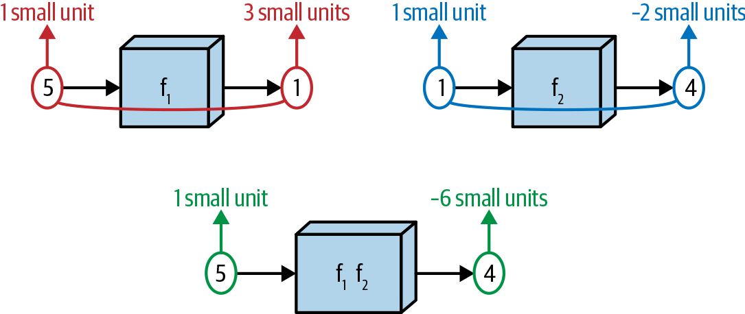
Figure 1-8. An illustration of the chain rule

Intuitively, using the diagram in Figure 1-8, the derivative of the composite function should be a sort of product of the derivatives of its constituent functions. Let’s say we feed the value 5 into the first function, and let’s say further that computing the derivative of the first function at u = 5 gives us a value of 3—that is, $\frac{d{f}_1}{du}\left(5\right)=3$.

Let’s say that we then take the value of the function that comes out of the first box—let’s suppose it is 1, so that f₁(5) = 1—and compute the derivative of the second function f₂ at this value: that is, $\frac{d{f}_2}{du}\left(1\right)$. We find that this value is –2.

If we think about these functions as being literally strung together, then if changing the input to box two by 1 unit yields a change of –2 units in the output of box two, changing the input to box two by 3 units should change the output to box two by –2 × 3 = –6 units. This is why in the formula for the chain rule, the final result is ultimately a product: $\frac{d{f}_2}{du}\left(f_1\left(x\right)\right)$ times $\frac{d{f}_1}{du}\left(x\right)$.

So by considering the diagram and the math, we can reason through what the derivative of the output of a nested function with respect to its input ought to be, using the chain rule. What might the code instructions for the computation of this derivative look like?

Code

Let’s code this up and show that computing derivatives in this way does in fact yield results that “look correct.” We’ll use the square function from “Basic functions in NumPy” along with sigmoid, another function that ends up being important in deep learning:

def sigmoid(x: ndarray) -> ndarray:
    '''
    Apply the sigmoid function to each element in the input ndarray.
    '''
    return 1 / (1 + np.exp(-x))

And now we code up the chain rule:

def chain_deriv_2(chain: Chain,
                  input_range: ndarray) -> ndarray:
    '''
    Uses the chain rule to compute the derivative of two nested functions:
    (f2(f1(x))' = f2'(f1(x)) * f1'(x)
    '''

    assert len(chain) == 2, \
    "This function requires 'Chain' objects of length 2"

    assert input_range.ndim == 1, \
    "Function requires a 1 dimensional ndarray as input_range"

    f1 = chain[0]
    f2 = chain[1]

    # df1/dx
    f1_of_x = f1(input_range)

    # df1/du
    df1dx = deriv(f1, input_range)

    # df2/du(f1(x))
    df2du = deriv(f2, f1(input_range))

    # Multiplying these quantities together at each point
    return df1dx * df2du

Figure 1-9 plots the results and shows that the chain rule works:

PLOT_RANGE = np.arange(-3, 3, 0.01)

chain_1 = [square, sigmoid]
chain_2 = [sigmoid, square]

plot_chain(chain_1, PLOT_RANGE)
plot_chain_deriv(chain_1, PLOT_RANGE)

plot_chain(chain_2, PLOT_RANGE)
plot_chain_deriv(chain_2, PLOT_RANGE)

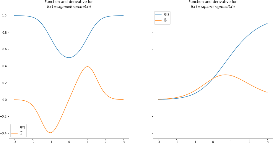
Figure 1-9. The chain rule works, part 1

The chain rule seems to be working. When the functions are upward-sloping, the derivative is positive; when they are flat, the derivative is zero; and when they are downward-sloping, the derivative is negative.

So we can in fact compute, both mathematically and via code, the derivatives of nested or “composite” functions such as f₁ f₂, as long as the individual functions are themselves mostly differentiable.

It will turn out that deep learning models are, mathematically, long chains of these mostly differentiable functions; spending time going manually through a slightly longer example in detail will help build your intuition about what is going on and how it can generalize to more complex models.

A Slightly Longer Example

Let’s closely examine a slightly longer chain: if we have three mostly differentiable functions—f₁, f₂, and f₃—how would we go about computing the derivative of f₁ f₂ f₃? We “should” be able to do it, since from the calculus theorem mentioned previously, we know that the composite of any finite number of “mostly differentiable” functions is differentiable.

Math

Mathematically, the result turns out to be the following expression:

$$\frac{d{f}_3}{du}\left(x\right)=\frac{d{f}_3}{du}\left(f_2\left(f_1\left(x\right)\right)\right)\times \frac{d{f}_2}{du}\left(f_1\left(x\right)\right)\times \frac{d{f}_1}{du}\left(x\right))$$

The underlying logic as to why the formula works for chains of length 2, $\frac{d{f}_2}{du}\left(x\right)=\frac{d{f}_2}{du}\left(f_1\left(x\right)\right)\times \frac{d{f}_1}{du}\left(x\right)$, also applies here—as does the lack of intuition from looking at the formula alone!

Diagram

The best way to (literally) see why this formula makes sense is via another box diagram, as shown in Figure 1-10.

Figure 1-10. The “box model” for computing the derivative of three nested functions

Using similar reasoning to the prior section: if we imagine the input to f₁ f₂ f₃ (call it a) being connected to the output (call it b) by a string, then changing a by a small amount Δ will result in a change in f₁(a) of $\frac{d{f}_1}{du}\left(x\right))$ times Δ, which will result in a change to $f_2\left(f_1\left(x\right)\right)$ (the next step along in the chain) of $\frac{d{f}_2}{du}\left(f_1\left(x\right)\right)\times \frac{d{f}_1}{du}\left(x\right))$ times Δ, and so on for the third step, when we get to the final change equal to the full formula for the preceding chain rule times Δ. Spend a bit of time going through this explanation and the earlier diagram—but not too much time, since we’ll develop even more intuition for this when we code it up.

Code

How might we translate such a formula into code instructions for computing the derivative, given the constituent functions? Interestingly, already in this simple example we see the beginnings of what will become the forward and backward passes of a neural network:

def chain_deriv_3(chain: Chain,
                  input_range: ndarray) -> ndarray:
    '''
    Uses the chain rule to compute the derivative of three nested functions:
    (f3(f2(f1)))' = f3'(f2(f1(x))) * f2'(f1(x)) * f1'(x)
    '''

    assert len(chain) == 3, \
    "This function requires 'Chain' objects to have length 3"

    f1 = chain[0]
    f2 = chain[1]
    f3 = chain[2]

    # f1(x)
    f1_of_x = f1(input_range)

    # f2(f1(x))
    f2_of_x = f2(f1_of_x)

    # df3du
    df3du = deriv(f3, f2_of_x)

    # df2du
    df2du = deriv(f2, f1_of_x)

    # df1dx
    df1dx = deriv(f1, input_range)

    # Multiplying these quantities together at each point
    return df1dx * df2du * df3du

Something interesting took place here—to compute the chain rule for this nested function, we made two “passes” over it:

1. First, we went “forward” through it, computing the quantities f1_of_x and f2_of_x along the way. We can call this (and think of it as) “the forward pass.”

2. Then, we “went backward” through the function, using the quantities that we computed on the forward pass to compute the quantities that make up the derivative.

Finally, we multiplied three of these quantities together to get our derivative.

Now, let’s show that this works, using the three simple functions we’ve defined so far: sigmoid, square, and leaky_relu.

PLOT_RANGE = np.range(-3, 3, 0.01)
plot_chain([leaky_relu, sigmoid, square], PLOT_RANGE)
plot_chain_deriv([leaky_relu, sigmoid, square], PLOT_RANGE)

Figure 1-11 shows the result.

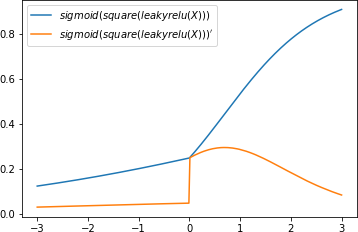
Figure 1-11. The chain rule works, even with triply nested functions

Again, comparing the plots of the derivatives to the slopes of the original functions, we see that the chain rule is indeed computing the derivatives properly.

Let’s now apply our understanding to composite functions with multiple inputs, a class of functions that follows the same principles we already established and is ultimately more applicable to deep learning.

Functions with Multiple Inputs

By this point, we have a conceptual understanding of how functions can be strung together to form composite functions. We also have a sense of how to represent these functions as series of boxes that inputs go into and outputs come out of. Finally, we’ve walked through how to compute the derivatives of these functions so that we understand these derivatives both mathematically and as quantities computed via a step-by-step process with a “forward” and “backward” component.

Oftentimes, the functions we deal with in deep learning don’t have just one input. Instead, they have several inputs that at certain steps are added together, multiplied, or otherwise combined. As we’ll see, computing the derivatives of the outputs of these functions with respect to their inputs is still no problem: let’s consider a very simple scenario with multiple inputs, where two inputs are added together and then fed through another function.

Math

For this example, it is actually useful to start by looking at the math. If our inputs are x and y, then we could think of the function as occurring in two steps. In Step 1, x and y are fed through a function that adds them together. We’ll denote that function as α (we’ll use Greek letters to refer to function names throughout) and the output of the function as a. Formally, this is simply:

$$a=\alpha (x,y)=x+y$$

Step 2 would be to feed a through some function σ (σ can be any continuous function, such as sigmoid, or the square function, or even a function whose name doesn’t start with s). We’ll denote the output of this function as s:

$$s=\sigma \left(a\right)$$

We could, equivalently, denote the entire function as f and write:

$$f(x,y)=\sigma (x+y)$$

This is more mathematically concise, but it obscures the fact that this is really two operations happening sequentially. To illustrate that, we need the diagram in the next section.

Diagram

Now that we’re at the stage where we’re examining functions with multiple inputs, let’s pause to define a concept we’ve been dancing around: the diagrams with circles and arrows connecting them that represent the mathematical “order of operations” can be thought of as computational graphs. For example, Figure 1-12 shows a computational graph for the function f we just described.

Figure 1-12. Function with multiple inputs

Here we see the two inputs going into α and coming out as a and then being fed through σ.

Code

Coding this up is very straightforward; note, however, that we have to add one extra assertion:

def multiple_inputs_add(x: ndarray,
                        y: ndarray,
                        sigma: Array_Function) -> float:
    '''
    Function with multiple inputs and addition, forward pass.
    '''
    assert x.shape == y.shape

    a = x + y
    return sigma(a)

Unlike the functions we saw earlier in this chapter, this function does not simply operate “elementwise” on each element of its input ndarrays. Whenever we deal with an operation that takes multiple ndarrays as inputs, we have to check their shapes to ensure they meet whatever conditions are required by that operation. Here, for a simple operation such as addition, all we need to check is that the shapes are identical so that the addition can happen elementwise.

Derivatives of Functions with Multiple Inputs

It shouldn’t seem surprising that we can compute the derivative of the output of such a function with respect to both of its inputs.

Diagram

Conceptually, we simply do the same thing we did in the case of functions with one input: compute the derivative of each constituent function “going backward” through the computational graph and then multiply the results together to get the total derivative. This is shown in Figure 1-13.

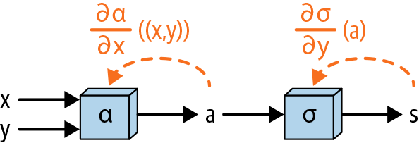
Figure 1-13. Going backward through the computational graph of a function with multiple inputs

Math

The chain rule applies to these functions in the same way it applied to the functions in the prior sections. Since this is a nested function, with $f(x,y)=\sigma \left(\alpha \right(x,y\left)\right)$, we have:

$$\frac{\partial f}{\partial x}=\frac{\partial \sigma }{\partial u}\left(\alpha (x,y)\right)\times \frac{\partial \alpha }{\partial x}\left((x,y)\right)=\frac{\partial \sigma }{\partial u}(x+y)\times \frac{\partial \alpha }{\partial x}\left((x,y)\right)$$

And of course $\frac{\partial f}{\partial y}$ would be identical.

Now note that:

$$\frac{\partial \alpha }{\partial x}\left((x,y)\right)=1$$

since for every unit increase in x, a increases by one unit, no matter the value of x (the same holds for y).

Given this, we can code up how we might compute the derivative of such a function.

Code

def multiple_inputs_add_backward(x: ndarray,
                                 y: ndarray,
                                 sigma: Array_Function) -> float:
    '''
    Computes the derivative of this simple function with respect to
    both inputs.
    '''
    # Compute "forward pass"
    a = x + y

    # Compute derivatives
    dsda = deriv(sigma, a)

    dadx, dady = 1, 1

    return dsda * dadx, dsda * dady

A straightforward exercise for the reader is to modify this for the case where x and y are multiplied instead of added.

Next, we’ll examine a more complicated example that more closely mimics what happens in deep learning: a similar function to the previous example, but with two vector inputs.

Functions with Multiple Vector Inputs

In deep learning, we deal with functions whose inputs are vectors or matrices. Not only can these objects be added, multiplied, and so on, but they can also combined via a dot product or a matrix multiplication. In the rest of this chapter, I’ll show how the mathematics of the chain rule and the logic of computing the derivatives of these functions using a forward and backward pass can still apply.

These techniques will end up being central to understanding why deep learning works. In deep learning, our goal will be to fit a model to some data. More precisely, this means that we want to find a mathematical function that maps observations from the data—which will be inputs to the function—to some desired predictions from the data—which will be the outputs of the function—in as optimal a way as possible. It turns out these observations will be encoded in matrices, typically with row as an observation and each column as a numeric feature for that observation. We’ll cover this in more detail in the next chapter; for now, being able to reason about the derivatives of complex functions involving dot products and matrix multiplications will be essential.

Let’s start by defining precisely what I mean, mathematically.

Math

A typical way to represent a single data point, or “observation,” in a neural network is as a row with n features, where each feature is simply a number x₁, x₂, and so on, up to x_n:

$$X=\left[\begin{array}{cccc}{x}_1& x_2& ...& x_n\end{array}\right]$$

A canonical example to keep in mind here is predicting housing prices, which we’ll build a neural network from scratch to do in the next chapter; in this example, x₁, x₂, and so on are numerical features of a house, such as its square footage or its proximity to schools.

Creating New Features from Existing Features

Perhaps the single most common operation in neural networks is to form a “weighted sum” of these features, where the weighted sum could emphasize certain features and de-emphasize others and thus be thought of as a new feature that itself is just a combination of old features. A concise way to express this mathematically is as a dot product of this observation, with some set of “weights” of the same length as the features, w₁, w₂, and so on, up to w_n. Let’s explore this concept from the three perspectives we’ve used thus far in this chapter.

Math

To be mathematically precise, if:

$$W=\left[\begin{array}{c}{w}_1\\ w_2\\ ⋮\\ w_n\end{array}\right]$$

then we could define the output of this operation as:

$$N=\nu (X,W)=X\times W=x_1\times w_1+x_2\times w_2+...+x_n\times w_n$$

Note that this operation is a special case of a matrix multiplication that just happens to be a dot product because X has one row and W has only one column.

Next, let’s look at a few ways we could depict this with a diagram.

Diagram

A simple way of depicting this operation is shown in Figure 1-14.

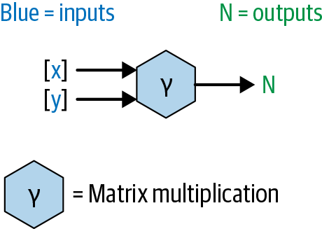
Figure 1-14. Diagram of a vector dot product

This diagram depicts an operation that takes in two inputs, both of which can be ndarrays, and produces one output ndarray.

But this is really a massive shorthand for many operations that are happening on many inputs. We could instead highlight the individual operations and inputs, as shown in Figures 1-15 and 1-16.

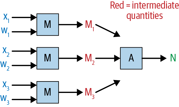
Figure 1-15. Another diagram of a matrix multiplication

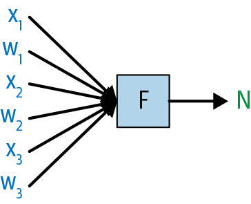
Figure 1-16. A third diagram of a matrix multiplication

The key point is that the dot product (or matrix multiplication) is a concise way to represent many individual operations; in addition, as we’ll start to see in the next section, using this operation makes our derivative calculations on the backward pass extremely concise as well.

Code

Finally, in code this operation is simply:

def matmul_forward(X: ndarray,
                   W: ndarray) -> ndarray:
    '''
    Computes the forward pass of a matrix multiplication.
    '''

    assert X.shape[1] == W.shape[0], \
    '''
    For matrix multiplication, the number of columns in the first array should
    match the number of rows in the second; instead the number of columns in the
    first array is {0} and the number of rows in the second array is {1}.
    '''.format(X.shape[1], W.shape[0])

    # matrix multiplication
    N = np.dot(X, W)

    return N

where we have a new assertion that ensures that the matrix multiplication will work. (This is necessary since this is our first operation that doesn’t merely deal with ndarrays that are the same size and perform an operation elementwise—our output is now actually a different size than our input.)

Derivatives of Functions with Multiple Vector Inputs

For functions that simply take one input as a number and produce one output, like f(x) = x² or f(x) = sigmoid(x), computing the derivative is straightforward: we simply apply rules from calculus. For vector functions, it isn’t immediately obvious what the derivative is: if we write a dot product as $\nu (X,W)=N$, as in the prior section, the question naturally arises—what would $\frac{\partial N}{\partial X}$ and $\frac{\partial N}{\partial W}$ be?

Diagram

Conceptually, we just want to do something like in Figure 1-17.

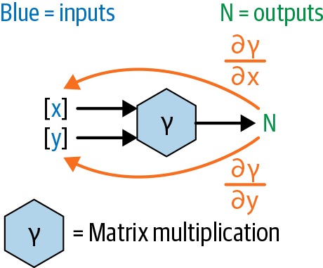
Figure 1-17. Backward pass of a matrix multiplication, conceptually

Calculating these derivatives was easy when we were just dealing with addition and multiplication, as in the prior examples. But how can we do the analogous thing with matrix multiplication? To define that precisely, we’ll have to turn to the math.

Math

First, how would we even define “the derivative with respect to a matrix”? Recalling that the matrix syntax is just shorthand for a bunch of numbers arranged in a particular form, “the derivative with respect to a matrix” really means “the derivative with respect to each element of the matrix.” Since X is a row, a natural way to define it is:

$$\frac{\partial \nu }{\partial X}=\left[\begin{array}{ccc}\frac{\partial \nu }{\partial x_1}& \frac{\partial \nu }{\partial x_2}& \frac{\partial \nu }{\partial x_3}\end{array}\right]$$

However, the output of ν is just a number: $N=x_1\times w_1+x_2\times w_2+x_3\times w_3$. And looking at this, we can see that if, for example, $x_1$ changes by ϵ units, then N will change by $w_1\times ϵ$ units—and the same logic applies to the other x_i elements. Thus:

$$\frac{\partial \nu }{\partial x_1}=w_1$$

$$\frac{\partial \nu }{\partial x_2}=w_2$$

$$\frac{\partial \nu }{\partial x_3}=w_3$$

And so:

$$\frac{\partial \nu }{\partial X}=\left[\begin{array}{ccc}{w}_1& w_2& w_3\end{array}\right]=W^T$$

This is a surprising and elegant result that turns out to be a key piece of the puzzle to understanding both why deep learning works and how it can be implemented so cleanly.

Using similar reasoning, we can see that:

$$\frac{\partial \nu }{\partial W}=\left[\begin{array}{c}{x}_1\\ x_2\\ x_3\end{array}\right]=X^T$$

Code

Here, reasoning mathematically about what the answer “should” be was the hard part. The easy part is coding up the result:

def matmul_backward_first(X: ndarray,
                          W: ndarray) -> ndarray:
    '''
    Computes the backward pass of a matrix multiplication with respect to the
    first argument.
    '''

    # backward pass
    dNdX = np.transpose(W, (1, 0))

    return dNdX

The dNdX quantity computed here represents the partial derivative of each element of X with respect to the sum of the output N. There is a special name for this quantity that we’ll use throughout the book: we’ll call it the gradient of X with respect to X. The idea is that for an individual element of X—say, x₃—the corresponding element in dNdx (dNdX[2], to be specific) is the partial derivative of the output of the vector dot product N with respect to x₃. The term “gradient” as we’ll use it in this book simply refers to a multidimensional analogue of the partial derivative; specifically, it is an array of partial derivatives of the output of a function with respect to each element of the input to that function.

Vector Functions and Their Derivatives: One Step Further

Deep learning models, of course, involve more than one operation: they include long chains of operations, some of which are vector functions like the one covered in the last section, and some of which simply apply a function elementwise to the ndarray they receive as input. Therefore, we’ll now look at computing the derivative of a composite function that includes both kinds of functions. Let’s suppose our function takes in the vectors X and W, performs the dot product described in the prior section—which we’ll denote as $\nu (X,W)$—and then feeds the vectors through a function σ. We’ll express the same objective as before, but in new language: we want to compute the gradients of the output of this new function with respect to X and W. Again, starting in the next chapter, we’ll see in precise detail how this is connected to what neural networks do, but for now we just want to build up the idea that we can compute gradients for computational graphs of arbitrary complexity.

Diagram

The diagram for this function, shown in Figure 1-18, is the same as in Figure 1-17, with the σ function simply added onto the end.

Figure 1-18. Same graph as before, but with another function tacked onto the end

Math

Mathematically, this is straightforward as well:

$$s=f(X,W)=\sigma \left(\nu (X,W)\right)=\sigma (x_1\times w_1+x_2\times w_2+x_3\times w_3)$$

Code

Finally, we can code this function up as:

def matrix_forward_extra(X: ndarray,
                         W: ndarray,
                         sigma: Array_Function) -> ndarray:
    '''
    Computes the forward pass of a function involving matrix multiplication,
    one extra function.
    '''
    assert X.shape[1] == W.shape[0]

    # matrix multiplication
    N = np.dot(X, W)

    # feeding the output of the matrix multiplication through sigma
    S = sigma(N)

    return S

Vector Functions and Their Derivatives: The Backward Pass

The backward pass is similarly just a straightforward extension of the prior example.

Math

Since f(X, W) is a nested function—specifically, f(X, W) = σ(ν(X, W))—its derivative with respect to, for example, X should conceptually be:

$$\frac{\partial f}{\partial X}=\frac{\partial \sigma }{\partial u}\left(\nu (X,W)\right)\times \frac{\partial \nu }{\partial X}(X,W)$$

But the first part of this is simply:

$$\frac{\partial \sigma }{\partial u}\left(\nu (X,W)\right)=\frac{\partial \sigma }{\partial u}(x_1\times w_1+x_2\times w_2+x_3\times w_3)$$

which is well defined since σ is just a continuous function whose derivative we can evaluate at any point, and here we are just evaluating it at $x_1\times w_1+x_2\times w_2+x_3\times w_3$.

Furthermore, we reasoned in the prior example that $\frac{\partial \nu }{\partial X}(X,W)=W^T$. Therefore:

$$\frac{\partial f}{\partial X}=\frac{\partial \sigma }{\partial u}\left(\nu (X,W)\right)\times \frac{\partial \nu }{\partial X}(X,W)=\frac{\partial \sigma }{\partial u}(x_1\times w_1+x_2\times w_2+x_3\times w_3)\times W^T$$

which, as in the preceding example, results in a vector of the same shape as X, since the final answer is a number, $\frac{\partial \sigma }{\partial u}(x_1\times w_1+x_2\times w_2+x_3\times w_3)$, times a vector of the same shape as X in W^T.

Diagram

The diagram for the backward pass of this function, shown in Figure 1-19, is similar to that of the prior example and even higher level than the math; we just have to add one more multiplication based on the derivative of the σ function evaluated at the result of the matrix multiplication.

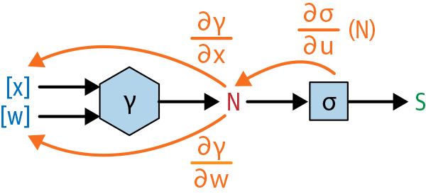
Figure 1-19. Graph with a matrix multiplication: the backward pass

Code

Finally, coding up the backward pass is straightforward as well:

def matrix_function_backward_1(X: ndarray,
                               W: ndarray,
                               sigma: Array_Function) -> ndarray:
    '''
    Computes the derivative of our matrix function with respect to
    the first element.
    '''
    assert X.shape[1] == W.shape[0]

    # matrix multiplication
    N = np.dot(X, W)

    # feeding the output of the matrix multiplication through sigma
    S = sigma(N)

    # backward calculation
    dSdN = deriv(sigma, N)

    # dNdX
    dNdX = np.transpose(W, (1, 0))

    # multiply them together; since dNdX is 1x1 here, order doesn't matter
    return np.dot(dSdN, dNdX)

Notice that we see the same dynamic here that we saw in the earlier example with the three nested functions: we compute quantities on the forward pass (here, just N) that we then use during the backward pass.

Is this right?

How can we tell if these derivatives we’re computing are correct? A simple test is to perturb the input a little bit and observe the resulting change in output. For example, X in this case is:

print(X)

[[ 0.4723  0.6151 -1.7262]]

If we increase x₃ by 0.01, from -1.726 to -1.716, we should see an increase in the value produced by the forward function of the gradient of the output with respect to x₃ × 0.01. Figure 1-20 shows this.

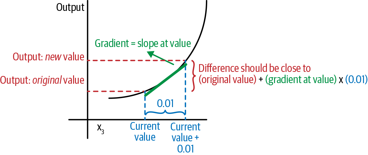
Figure 1-20. Gradient checking: an illustration

Using the matrix_function_backward_1 function, we can see that the gradient is -0.1121:

print(matrix_function_backward_1(X, W, sigmoid))

[[ 0.0852 -0.0557 -0.1121]]

To test whether this gradient is correct, we should see, after incrementing x₃ by 0.01, a corresponding decrease in the output of the function by about 0.01 × -0.1121 = -0.001121; if we saw an decrease by more or less than this amount, or an increase, for example, we would know that our reasoning about the chain rule was off. What we see when we do this calculation,² however, is that increasing x₃ by a small amount does indeed decrease the value of the output of the function by 0.01 × -0.1121—which means the derivatives we’re computing are correct!

To close out this chapter, we’ll cover an example that builds on everything we’ve done so far and directly applies to the models we’ll build in the next chapter: a computational graph that starts by multiplying a pair of two-dimensional matrices together.

Computational Graph with Two 2D Matrix Inputs

In deep learning, and in machine learning more generally, we deal with operations that take as input two 2D arrays, one of which represents a batch of data X and the other of which represents the weights W. In the next chapter, we’ll dive deep into why this makes sense in a modeling context, but in this chapter we’ll just focus on the mechanics and the math behind this operation. Specifically. we’ll walk through a simple example in detail and show that even when multiplications of 2D matrices are involved, rather than just dot products of 1D vectors, the reasoning we’ve been using throughout this chapter still makes mathematical sense and is in fact extremely easy to code.

As before, the math needed to derive these results gets…not difficult, but messy. Nevertheless, the result is quite clean. And, of course, we’ll break it down step by step and always connect it back to both code and diagrams.

Math

Let’s suppose that:

$$X=\left[\begin{array}{ccc}{x}_{11}& x_{12}& x_{13}\\ x_{21}& x_{22}& x_{23}\\ x_{31}& x_{32}& x_{33}\end{array}\right]$$

and:

$$W=\left[\begin{array}{cc}{w}_{11}& w_{12}\\ w_{21}& w_{22}\\ w_{31}& w_{32}\end{array}\right]$$

This could correspond to a dataset in which each observation has three features, and the three rows could correspond to three different observations for which we want to make predictions.

Now we’ll define the following straightforward operations to these matrices:

1. Multiply these matrices together. As before, we’ll denote the function that does this as ν(X, W) and the output as N, so that N = ν(X, W).

2. Feed $N$ result through some differentiable function σ, and define (S = σ(N).

As before, the question now is: what are the gradients of the output S with respect to X and W? Can we simply use the chain rule again? Why or why not?

If you think about this for a bit, you may realize that something is different from the previous examples that we’ve looked at: S is now a matrix, not simply a number. And what, after all, does the gradient of one matrix with respect to another matrix mean?

This leads us to a subtle but important idea: we may perform whatever series of operations on multidimensional arrays we want, but for the notion of a “gradient” with respect to some output to be well defined, we need to sum (or otherwise aggregate into a single number) the final array in the sequence so that the notion of “how much will changing each element of X affect the output” will even make sense.

So we’ll tack onto the end a third function, Lambda, that simply takes the elements of S and sums them up.

Let’s make this mathematically concrete. First, let’s multiply X and W:

$$X\times W=\left[\begin{array}{cc}{x}_{11}\times w_{11}+x_{12}\times w_{21}+x_{13}\times w_{31}& x_{11}\times w_{12}+x_{12}\times w_{22}+x_{13}\times w_{32}\\ x_{21}\times w_{11}+x_{22}\times w_{21}+x_{23}\times w_{31}& x_{21}\times w_{12}+x_{22}\times w_{22}+x_{23}\times w_{32}\\ x_{31}\times w_{11}+x_{32}\times w_{21}+x_{33}\times w_{31}& x_{31}\times w_{12}+x_{32}\times w_{22}+x_{33}\times w_{32}\end{array}\right]=\left[\begin{array}{cc}X{W}_{11}& X{W}_{12}\\ X{W}_{21}& X{W}_{22}\\ X{W}_{31}& X{W}_{32}\end{array}\right]$$

where we denote row i and column j in the resulting matrix as $X{W}_{ij}$ for convenience.

Next, we’ll feed this result through σ, which just means applying σ to every element of the matrix $X\times W$:

$$\sigma (X\times W)=\left[\begin{array}{cc}\sigma (x_{11}\times w_{11}+x_{12}\times w_{21}+x_{13}\times w_{31})& \sigma (x_{11}\times w_{12}+x_{12}\times w_{22}+x_{13}\times w_{32})\\ \sigma (x_{21}\times w_{11}+x_{22}\times w_{21}+x_{23}\times w_{31})& \sigma (x_{21}\times w_{12}+x_{22}\times w_{22}+x_{23}\times w_{32})\\ \sigma (x_{31}\times w_{11}+x_{32}\times w_{21}+x_{33}\times w_{31})& \sigma (x_{31}\times w_{12}+x_{32}\times w_{22}+x_{33}\times w_{32})\end{array}\right]=\left[\begin{array}{cc}\sigma \left(X{W}_{11}\right)& \sigma \left(X{W}_{12}\right)\\ \sigma \left(X{W}_{21}\right)& \sigma \left(X{W}_{22}\right)\\ \sigma \left(X{W}_{31}\right)& \sigma \left(X{W}_{32}\right)\end{array}\right]$$

Finally, we can simply sum up these elements:

$$L=\Lambda \left(\sigma (X\times W)\right)=\Lambda \left(\left[\begin{array}{cc}\sigma \left(X{W}_{11}\right)& \sigma \left(X{W}_{12}\right)\\ \sigma \left(X{W}_{21}\right)& \sigma \left(X{W}_{22}\right)\\ \sigma \left(X{W}_{31}\right)& \sigma \left(X{W}_{32}\right)\end{array}\right]\right)=\sigma \left(X{W}_{11}\right)+\sigma \left(X{W}_{12}\right)+\sigma \left(X{W}_{21}\right)+\sigma \left(X{W}_{22}\right)+\sigma \left(X{W}_{31}\right)+\sigma \left(X{W}_{32}\right)$$

Now we are back in a pure calculus setting: we have a number, L, and we want to figure out the gradient of L with respect to X and W; that is, we want to know how much changing each element of these input matrices (x₁₁, w₂₁, and so on) would change L. We can write this as:

$$\frac{\partial \Lambda }{\partial u}\left(X\right)=\left[\begin{array}{ccc}\frac{\partial \Lambda }{\partial u}\left(x_{11}\right)& \frac{\partial \Lambda }{\partial u}\left(x_{12}\right)& \frac{\partial \Lambda }{\partial u}\left(x_{13}\right)\\ \frac{\partial \Lambda }{\partial u}\left(x_{21}\right)& \frac{\partial \Lambda }{\partial u}\left(x_{22}\right)& \frac{\partial \Lambda }{\partial u}\left(x_{23}\right)\\ \frac{\partial \Lambda }{\partial u}\left(x_{31}\right)& \frac{\partial \Lambda }{\partial u}\left(x_{32}\right)& \frac{\partial \Lambda }{\partial u}\left(x_{33}\right)\end{array}\right]$$

And now we understand mathematically the problem we are up against. Let’s pause the math for a second and catch up with our diagram and code.

Diagram

Conceptually, what we are doing here is similar to what we’ve done in the previous examples with a computational graph with multiple inputs; thus, Figure 1-21 should look familiar.

Figure 1-21. Graph of a function with a complicated forward pass

We are simply sending inputs forward as before. We claim that even in this more complicated scenario, we should be able to calculate the gradients we need using the chain rule.

Code

We can code this up as:

def matrix_function_forward_sum(X: ndarray,
                                W: ndarray,
                                sigma: Array_Function) -> float:
    '''
    Computing the result of the forward pass of this function with
    input ndarrays X and W and function sigma.
    '''
    assert X.shape[1] == W.shape[0]

    # matrix multiplication
    N = np.dot(X, W)

    # feeding the output of the matrix multiplication through sigma
    S = sigma(N)

    # sum all the elements
    L = np.sum(S)

    return L

The Fun Part: The Backward Pass

Now we want to “perform the backward pass” for this function, showing how, even when a matrix multiplication is involved, we can end up calculating the gradient of N with respect to each of the elements of our input ndarrays.³ With this final step figured out, starting to train real machine learning models in Chapter 2 will be straightforward. First, let’s remind ourselves what we are doing, conceptually.

Diagram

Again, what we’re doing is similar to what we’ve done in the prior examples from this chapter; Figure 1-22 should look as familiar as Figure 1-21 did.

Figure 1-22. Backward pass through our complicated function

We simply need to calculate the partial derivative of each constituent function and evaluate it at its input, multiplying the results together to get the final derivative. Let’s consider each of these partial derivatives in turn; the only way through it is through the math.

Math

Let’s first note that we could compute this directly. The value L is indeed a function of x₁₁, x₁₂, and so on, all the way up to x₃₃.

However, that seems complicated. Wasn’t the whole point of the chain rule that we can break down the derivatives of complicated functions into simple pieces, compute each of those pieces, and then just multiply the results? Indeed, that fact was what made it so easy to code these things up: we just went step by step through the forward pass, saving the results as we went, and then we used those results to evaluate all the necessary derivatives for the backward pass.

I’ll show that this approach only kind of works when there are matrices involved. Let’s dive in.

We can write L as $\Lambda \left(\sigma \right(\nu (X,W)\left)\right)$. If this were a regular function, we would just write the chain rule:

$$\frac{\partial \Lambda }{\partial X}\left(X\right)=\frac{\partial \nu }{\partial X}(X,W)\times \frac{\partial \sigma }{\partial u}\left(N\right)\times \frac{\partial \Lambda }{\partial u}\left(S\right)$$

Then we would compute each of the three partial derivatives in turn. This is exactly what we did before in the function of three nested functions, for which we computed the derivative using the chain rule, and Figure 1-22 suggests that approach should work for this function as well.

The first derivative is the most straightforward and thus makes the best warm-up. We want to know how much L (the output of Λ) will increase if each element of S increases. Since L is the sum of all the elements of S, this derivative is simply:

$$\frac{\partial \Lambda }{\partial u}\left(S\right)=\left[\begin{array}{cc}1& 1\\ 1& 1\\ 1& 1\end{array}\right]$$

since increasing any element of S by, say, 0.46 units would increase Λ by 0.46 units.

Next, we have $\frac{\partial \sigma }{\partial u}\left(N\right)$. This is simply the derivative of whatever function σ is, evaluated at the elements in N. In the "XW" syntax we’ve used previously, this is again simple to compute:

$$\left[\begin{array}{cc}\frac{\partial \sigma }{\partial u}\left(X{W}_{11}\right)& \frac{\partial \sigma }{\partial u}\left(X{W}_{12}\right)\\ \frac{\partial \sigma }{\partial u}\left(X{W}_{21}\right)& \frac{\partial \sigma }{\partial u}\left(X{W}_{22}\right)\\ \frac{\partial \sigma }{\partial u}\left(X{W}_{31}\right)& \frac{\partial \sigma }{\partial u}\left(X{W}_{32}\right)\end{array}\right]$$

Note that at this point we can say for certain that we can multiply these two derivatives together elementwise and compute $\frac{\partial L}{\partial u}\left(N\right)$:

$$\frac{\partial \Lambda }{\partial u}\left(N\right)=\frac{\partial \Lambda }{\partial u}\left(S\right)\times \frac{\partial \sigma }{\partial u}\left(N\right)=\left[\begin{array}{cc}\frac{\partial \sigma }{\partial u}\left(X{W}_{11}\right)& \frac{\partial \sigma }{\partial u}\left(X{W}_{12}\right)\\ \frac{\partial \sigma }{\partial u}\left(X{W}_{21}\right)& \frac{\partial \sigma }{\partial u}\left(X{W}_{22}\right)\\ \frac{\partial \sigma }{\partial u}\left(X{W}_{31}\right)& \frac{\partial \sigma }{\partial u}\left(X{W}_{32}\right)\end{array}\right]\times \left[\begin{array}{cc}1& 1\\ 1& 1\\ 1& 1\end{array}\right]=\left[\begin{array}{cc}\frac{\partial \sigma }{\partial u}\left(X{W}_{11}\right)& \frac{\partial \sigma }{\partial u}\left(X{W}_{12}\right)\\ \frac{\partial \sigma }{\partial u}\left(X{W}_{21}\right)& \frac{\partial \sigma }{\partial u}\left(X{W}_{22}\right)\\ \frac{\partial \sigma }{\partial u}\left(X{W}_{31}\right)& \frac{\partial \sigma }{\partial u}\left(X{W}_{32}\right)\end{array}\right]$$

Now, however, we are stuck. The next thing we want, based on the diagram and applying the chain rule, is $\frac{\partial \nu }{\partial u}\left(X\right)$. Recall, however, that N, the output of ν, was just the result of a matrix multiplication of X with W. Thus we want some notion of how much increasing each element of X (a 3 × 3 matrix) will increase each element of N (a 3 × 2 matrix). If you’re having trouble wrapping your mind around such a notion, that’s the point—it isn’t clear at all how we’d define this, or whether it would even be useful if we did.

Why is this a problem now? Before, we were in the fortunate situation of X and W being transposes of each other in terms of shape. That being the case, we could show that $\frac{\partial \nu }{\partial u}\left(X\right)=W^T$ and $\frac{\partial \nu }{\partial u}\left(W\right)=X^T$. Is there something analogous we can say here?

The “?”

More specifically, here’s where we’re stuck. We need to figure out what goes in the “?”:

$$\frac{\partial \Lambda }{\partial u}\left(X\right)=\frac{\partial \Lambda }{\partial u}\left(\sigma \left(N\right)\right)\times ?=\left[\begin{array}{cc}\frac{\partial \sigma }{\partial u}\left(X{W}_{11}\right)& \frac{\partial \sigma }{\partial u}\left(X{W}_{12}\right)\\ \frac{\partial \sigma }{\partial u}\left(X{W}_{21}\right)& \frac{\partial \sigma }{\partial u}\left(X{W}_{22}\right)\\ \frac{\partial \sigma }{\partial u}\left(X{W}_{31}\right)& \frac{\partial \sigma }{\partial u}\left(X{W}_{32}\right)\end{array}\right]\times ?$$

The answer

It turns out that because of the way the multiplication works out, what fills the “?” is simply W^T, as in the simpler example with the vector dot product that we just saw! The way to verify this is to compute the partial derivative of L with respect to each element of X directly; when we do so,⁴ the resulting matrix does indeed (remarkably) factor out into:

$$\frac{\partial \Lambda }{\partial u}\left(X\right)=\frac{\partial \Lambda }{\partial u}\left(S\right)\times \frac{\partial \sigma }{\partial u}\left(N\right)\times W^T$$

where the first multiplication is elementwise, and the second one is a matrix multiplication.

This means that even if the operations in our computational graph involve multiplying matrices with multiple rows and columns, and even if the shapes of the outputs of those operations are different than those of the inputs, we can still include these operations in our computational graph and backpropagate through them using “chain rule” logic. This is a critical result, without which training deep learning models would be much more cumbersome, as you’ll appreciate further after the next chapter.

Code

Let’s encapsulate what we just derived using code, and hopefully solidify our understanding in the process:

def matrix_function_backward_sum_1(X: ndarray,
                                   W: ndarray,
                                   sigma: Array_Function) -> ndarray:
    '''
    Compute derivative of matrix function with a sum with respect to the
    first matrix input.
    '''
    assert X.shape[1] == W.shape[0]

    # matrix multiplication
    N = np.dot(X, W)

    # feeding the output of the matrix multiplication through sigma
    S = sigma(N)

    # sum all the elements
    L = np.sum(S)

    # note: I'll refer to the derivatives by their quantities here,
    # unlike the math, where we referred to their function names

    # dLdS - just 1s
    dLdS = np.ones_like(S)

    # dSdN
    dSdN = deriv(sigma, N)

    # dLdN
    dLdN = dLdS * dSdN

    # dNdX
    dNdX = np.transpose(W, (1, 0))

    # dLdX
    dLdX = np.dot(dSdN, dNdX)

    return dLdX

Now let’s verify that everything worked:

np.random.seed(190204)
X = np.random.randn(3, 3)
W = np.random.randn(3, 2)

print("X:")
print(X)

print("L:")
print(round(matrix_function_forward_sum(X, W, sigmoid), 4))
print()
print("dLdX:")
print(matrix_function_backward_sum_1(X, W , sigmoid))

X:
[[-1.5775 -0.6664  0.6391]
 [-0.5615  0.7373 -1.4231]
 [-1.4435 -0.3913  0.1539]]
L:
2.3755

dLdX:
[[ 0.2489 -0.3748  0.0112]
 [ 0.126  -0.2781 -0.1395]
 [ 0.2299 -0.3662 -0.0225]]

As in the previous example, since dLdX represents the gradient of X with respect to L, this means that, for instance, the top-left element indicates that $\frac{\partial \Lambda }{\partial x_{11}}(X,W)=0.2489$. Thus, if the matrix math for this example was correct, then increasing x₁₁ by 0.001 should increase L by 0.01 × 0.2489. Indeed, we see that this is what happens:

X1 = X.copy()
X1[0, 0] += 0.001

print(round(
        (matrix_function_forward_sum(X1, W, sigmoid) - \
         matrix_function_forward_sum(X, W, sigmoid)) / 0.001, 4))

0.2489

Looks like the gradients were computed correctly!

Describing these gradients visually

To bring this back to what we noted at the beginning of the chapter, we fed the element in question, x₁₁, through a function with many operations: there was a matrix multiplication—which was really shorthand for combining the nine inputs in the matrix X with the six inputs in the matrix W to create six outputs—the sigmoid function, and then the sum. Nevertheless, we can also think of this as a single function called, say, "$WNSL$, “as depicted in Figure 1-23.

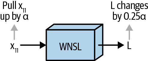
Figure 1-23. Another way of describing the nested function: as one function, “WNSL”

Since each function is differentiable, the whole thing is just a single differentiable function, with x₁₁ as an input; thus, the gradient is simply the answer to the question, what is $\frac{dL}{d{x}_{11}}$? To visualize this, we can simply plot how L changes as x₁₁ changes. Looking at the initial value of x₁₁, we see that it is -1.5775:

print("X:")
print(X)

X:
[[-1.5775 -0.6664  0.6391]
 [-0.5615  0.7373 -1.4231]
 [-1.4435 -0.3913  0.1539]]

If we plot the value of L that results from feeding X and W into the computational graph defined previously—or, to represent it differently, from feeding X and W into the function called in the preceding code—changing nothing except the value for x₁₁ (or X[0, 0]), the resulting plot looks like Figure 1-24.⁵

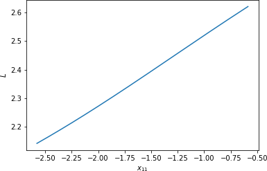
Figure 1-24. L versus x₁₁, holding other values of X and W constant

Indeed, eyeballing this relationship in the case of x₁₁, it looks like the distance this function increases along the L-axis is roughly 0.5 (from just over 2.1 to just over 2.6), and we know that we are showing a change of 2 along the x₁₁-axis, which would make the slope roughly $\frac{0.5}{2}=0.25$—which is exactly what we just calculated!

So our complicated matrix math does in fact seem to have resulted in us correctly computing the partial derivative L with respect to each element of X. Furthermore, the gradient of L with respect to W could be computed similarly.

Note

The expression for the gradient of L with respect to W would be X^T. However, because of the order in which the X^T expression factors out of the derivative for L, X^T would be on the left side of the expression for the gradient of L with respect to W:

$$\frac{\partial \Lambda }{\partial u}\left(W\right)=X^T\times \frac{\partial \Lambda }{\partial u}\left(S\right)\times \frac{\partial \sigma }{\partial u}\left(N\right)$$

In code, therefore, while we would have dNdW = np.transpose(X, (1, 0)), the next step would be:

dLdW = np.dot(dNdW, dSdN)

instead of dLdX = np.dot(dSdN, dNdX) as before.

Conclusion

After this chapter, you should have confidence that you can understand complicated nested mathematical functions and reason out how they work by conceptualizing them as a series of boxes, each one representing a single constituent function, connected by strings. Specifically, you can write code to compute the derivatives of the outputs of such functions with respect to any of the inputs, even when there are matrix multiplications involving two-dimensional ndarrays involved, and understand the math behind why these derivative computations are correct. These foundational concepts are exactly what we’ll need to start building and training neural networks in the next chapter, and to build and train deep learning models from scratch in the chapters after that. Onward!

¹ This will allow us to easily add a bias to our matrix multiplication later on.

² Throughout I’ll provide links to relevant supplementary material on a GitHub repo that contains the code for the book, including for this chapter.

³ In the following section we’ll focus on computing the gradient of N with respect to X, but the gradient with respect to W could be reasoned through similarly.

⁴ We do this in “Matrix Chain Rule”.

⁵ The full function can be found on the book’s website; it is simply a subset of the matrix function backward sum function shown on the previous page.