Design Patterns for Cloud Native Applications

Chapter 4. Data Management Patterns

Data is the key for all applications. Even a simple echo service depends on the data in the incoming message in order to send a response. This chapter is all about data and its management in cloud native applications.

First, we’ll focus on data architecture, explaining how data is collected, processed, and stored in cloud native applications. Then, we’ll look at understanding data by categorizing it through multiple dimensions, based on how it is used in an application, its structure, and its scale. We’ll discuss possible storage and processing options and how to make the best choice given a specific type of data.

We’ll then move on to explaining various patterns related to data, focusing on centralized and decentralized data, data composition, caching, management, performance optimization, reliability, and security. The chapter also covers various technologies currently used in the industry to effectively implement these cloud native applications’ development patterns.

This knowledge of data, patterns, and technologies together will help you design cloud native applications for your specific use case and for the type of data that your applications deal with.

Data Architecture

Cloud native applications should be able to collect, store, process, and present data in a way that fulfills our use cases (Figure 4-1).

Here, data sources are cloud native applications that feed data such as user inputs and sensor readings. They sometimes feed data into data-ingestion systems such as message brokers or, when possible, directly write to data stores. Data-ingestion systems can transfer data as events/messages to other applications or data stores; through these we will be able to achieve reliable and asynchronous data processing. (Chapter 5 provides more details about data-ingestion systems.)

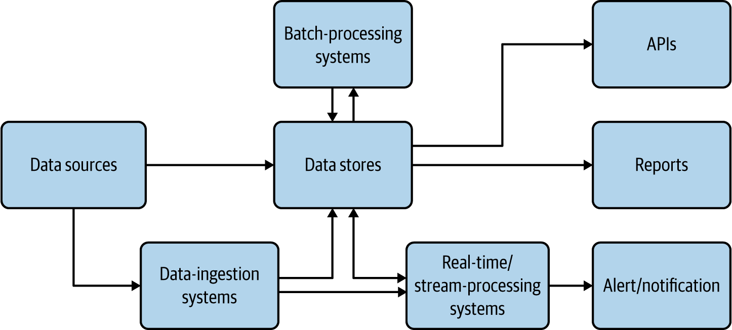
Figure 4-1. Data architecture for cloud native applications

The data stores are the critical part of this architecture; they store data in various formats and at scale to facilitate the use case. They are used as the source for generating reports and also used as the base of data APIs. We present more detail about data stores in the following sections.

Real-time and stream-processing systems process events on the fly and produce useful insights for the use case, as well as provide alerts and notifications when they happen. Chapter 6 covers these in detail. Batch-processing systems process data from data sources in batches, and write the processed output back to the data stores so it can be used for reporting or exposed via APIs. In these cases, the processing system may be reading data from one type of store and writing to another, such as reading from a filesystem and writing to a relational database. Batch processing of cloud native data is similar to traditional batch data processing, so we do not go into the details here.

Just as cloud native microservices have characteristics such as being scalable, resilient, and manageable, cloud native data has its own unique characteristics that are quite different from traditional data processing practices. Most important, cloud native data can be stored in many forms, in a variety of data formats and data stores. They are not expected to maintain a fixed schema and are encouraged to have duplicate data to facilitate availability and performance over consistency. Furthermore, in cloud native applications, multiple services are not encouraged to access the same database; instead, they should call respective service APIs that own the data store to access the data. All these provide separation of concerns and allow cloud native data to scale out.

Types and Forms of Data

Data, in its multiple forms, has a huge influence on applications—cloud native or not. This section discusses how data alters the execution of an application, the formats of this data, and how data can be best transmitted and stored.

Application behavior is influenced by the following three main types of data:

Input data

Sent as part of the input message by the user or client. Most commonly, this data is either JSON or XML messages, though binary formats such as gRPC and Thrift are getting some traction.

Configuration data

Provided by the environment as variables. XML has been used as the configuration language for a long time, and now YAML configs have become the de facto standard for cloud native applications.

State data

The data stored by the application itself, regarding its status, based on all messages and events that occurred before the current time. By persisting the state data and loading it on startup, the application will be able to seamlessly resume its functionality upon restart.

Applications that depend only on input and configuration (config) data are called stateless applications. These applications are relatively simple to implement and scale because their failure or restart has almost no impact on their execution. In contrast, applications that depend on input, config, and state data—stateful applications—are much more complex to implement and scale. The state of the application is stored in data stores, so application failures can result in partial writes that corrupt their state, which can lead to incorrect execution of the application.

Cloud native applications fall into both stateful and stateless categories. Chapter 3 covered stateless applications. This chapter focuses on stateful applications.

Cloud native applications use various forms of data, which are generally grouped into the following three categories:

Structured data

Can fit a predefined schema. For example, the data on a typical user registration form can be comfortably stored in a relational database.

Semi-structured data

Has some form of structure. For example, each field in a data entry may have a corresponding key or name that we can use to refer to it, but when we take all the entries, there is no guarantee that each entry will have the same number of fields or even common keys. This data can be easily represented through JSON, XML, and YAML formats.

Unstructured data

Does not contain any meaningful fields. Images, videos, and raw text content are examples. Usually, this data is stored without any understanding of its content.

Data Stores

We have to choose the data store type for cloud native data, based on the use case of the application. Different use cases use different types of data (structured, semi-structured, or unstructured) and have varying scalability and availability requirements. With the diverse storage options available, different data stores provide different characteristics, such as one providing high performance while another provides high scalability. At times we may even end up using more than one data store at the same time to achieve different characteristics. In this section, we look at common types of data stores, and when and how they can be used in cloud native applications.

Relational Databases

Relational databases are ideal for storing structured data that has a predefined schema. These databases use Structured Query Language (SQL) for processing, storing, and accessing data. They also follow the principle of defining schema on write: the data schema is defined before writing the data to the database.

Relational databases can optimally store and retrieve data by using database indexing and normalization. Because these databases support atomicity, consistency, isolation, and durability (ACID) properties, they can also provide transaction guarantees. Here, atomicity guarantees that all operations within a transaction are executed as a single unit; consistency ensures that the data is consistent before and after the transaction; isolation makes the intermediate state of a transaction invisible to other transactions; and, finally, durability guarantees that after a successful transaction, the data is persistent even in the event of a system failure. All these characteristics make relational databases ideal for implementing business-critical financial applications.

Relational databases do not work well with semi-structured data. For example, if we are storing product catalog data for an ecommerce site and the initial input contains product detail, price, some images, and reviews, we can’t store all this data in a relational store. Here we need to extract only the most important and common fields such as product ID, name, detail, and price to store in a relational database, while storing the list of product reviews in NoSQL and images in a filesystem. However, this approach could impose performance degradation due to multiple lookups when retrieving all the data. In such cases, we recommend storing critical unstructured and semi-structured data fields such as the product thumbnail image as a blob or text in the relational data store to improve read performance. When taking this approach, always consider the cost and space consumption of relational databases.

Relational databases are a good option for storing cloud native application data. We recommend using a relational database per microservice, as this will help deploy and scale the data along with the microservice as a single deployment unit. It is important to remember that relational databases are not scalable by design. In terms of scaling, they can support only primary/secondary architecture, allowing one node for write operations while having multiple worker nodes for read operations.

Therefore, we recommend using relational databases in cloud native applications when the number of records in the store will never exceed the limit that the database can efficiently process. If we can foresee that the data will constantly grow, such as with the number of orders, logs, or notifications stored, then we may need to deploy data-scaling patterns to relational data stores that we discuss later in this chapter, or we should look for other alternatives.

NoSQL Databases

The term NoSQL is usually misunderstood as not SQL. Rather, it is better explained as not only SQL. This is because these databases still have some good SQL-like query support and behaviors along with many other benefits, such as scalability, and the ability to store and process semi-structured data. NoSQL databases follow the principle of schema on read: the schema of the data is defined only at the time of accessing the data for processing, and not when it is written to the disk.

These databases are best suited to handling big data, as they are designed for scalability and performance. As NoSQL stores are distributed in nature, we can use them across multiple cloud native applications. To optimize performance, data stored in NoSQL databases is usually not normalized and can have redundant fields. When the data is normalized, table joins will need to be performed when retrieving data, and this can be time-consuming because of the distributed nature of these databases. Further, only a few NoSQL stores support transactions while compromising their performance and scalability; therefore, it is generally not recommended to store data in NoSQL stores that need transaction guarantees.

The usage of NoSQL stores in cloud native applications varies, as there are various types of NoSQL stores, and unlike relational databases, they do not have behavioral commonalities. These NoSQL stores can be categorized by the way they store data and by the consistency and availability guarantees they provide.

Some common NoSQL stores categorized by the way they store data are as follows:

Key-value store

This holds records as key-value pairs. We can use this for storing login session information based on session IDs. These types of stores are heavily used for caching data. Redis is one popular open source key-value data stores. Memcached and Ehcache are other popular options.

Column store

This stores multiple key (column) and value pairs in each of its rows, as shown in Figure 4-2. These stores are a good example of schema on read: we can write any number of columns during the write phase, and when data is retrieved, we can specify only the columns we are interested in processing. The most widely used column store is Apache Cassandra. For those who use big data and Apache Hadoop infrastructure, Apache HBase can be an option as it is part of the Hadoop ecosystem.

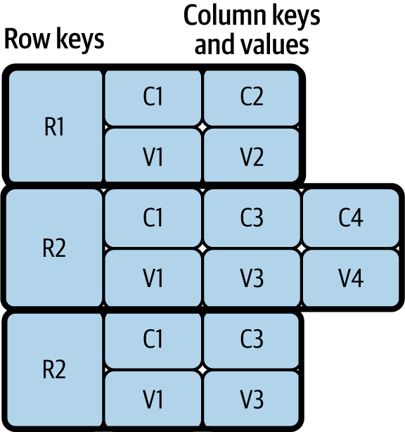
Figure 4-2. Column store

Document store

This can store semi-structured data such as JSON and XML documents. This also allows us to process stored documents by using JSON and XML path expressions. These data stores are popular as they can store JSON and XML messages, which are usually used by frontend applications and APIs for communication. MongoDB, Apache CouchDB, and CouchBase are popular options for storing JSON documents.

Graph store

These store data as nodes and use edges to represent the relationship between data nodes. These stores are multidimensional and are useful for building and querying networks such as networks of friends in social media and transaction networks for detecting fraud. Neo4j, the most popular graph data store, is heavily used by industry leaders.

Many other types of NoSQL stores, including object stores and time-series data stores, can help store and query use-case-specific specialized data. Some stores also have multimodel behavior; they can fall into several of the preceding categories. For example, Amazon DynamoDB can work as a key-value and document store, and Azure Cosmos DB can work as a key-value, column, document, and graph store.

NoSQL stores are distributed, so they need to adhere to the CAP theorem; CAP stands for consistency, availability, and partition tolerance. This theorem states that a distributed application can provide either full availability or consistency; we cannot achieve both while providing network partition tolerance. Here, availability means that the system is fully functional when some of its nodes are down, consistency means an update/change in one node is immediately propagated to other nodes, and partition tolerance means that the system can continue to work even when some nodes cannot connect to each other. Some stores prioritize consistency over availability, while others prioritize availability over consistency.

Say we need to keep track of and report the number of citizens in the country, and missing the latest data in the calculation will not cause significant error in the final outcome. We can use a data store that favors availability. On the other hand, when we need to track transactions for business purposes, we need to choose a data store that favors consistency.

Table 4-1 categorizes NoSQL data stores in terms of consistency and availability.

Table 4-1. NoSQL data stores favoring consistency and availability

	Favor consistency	Favor availability
Key-value stores	Redis, Memcached	DynamoDB, Voldemort
Column stores	Google Cloud Bigtable, Apache HBase	Apache Cassandra
Document stores	MongoDB, Terrastore	CouchDB, SimpleDB
Graph stores	Azure Cosmos DB	Neo4j

Though some favor consistency and others favor availability, still other NoSQL data stores (such as Cassandra and DynamoDB) can provide both. For example, in Cassandra we can define consistency levels such as One, Quorum, or All. When the consistency level is set to One, data is read/written to only one node in the cluster, providing full availability with eventual consistency. During eventual consistency, data is eventually propagated to other nodes, and reads can be outdated during this period. On the other hand, when set to All, data is read/written from all nodes before the operation succeeds, providing strong consistency with performance degradation. But when using Quorum, it reads/writes data from only 51% of the nodes. Through this, we can ensure that the latest update will be available in at least one node, providing both consistency and availability with a minimum performance overhead.

Therefore, we recommend that you understand the nature of the data and its use cases within cloud native applications before choosing the right NoSQL data store. Remember that the data format, as well as the consistency and availability requirements of the data, can influence your choice of data store.

Filesystem Storage

Filesystem storage is the best for storing unstructured data in cloud native applications. Unlike NoSQL stores, it does not try to understand the data but rather purely optimizes data storage and retrieval. We can also use filesystem storage to store large application data as a cache, as it can be cheaper than retrieving data repeatedly over the network.

Though this is the cheapest option, it may not be an optimal solution when storing text or semi-structured data, as this will force us to load multiple files when searching for a single data entry. In these cases, we recommend using indexing systems such as Apache Solr or Elasticsearch to facilitate search.

When data needs to be stored at scale, distributed filesystems can be used. The most well-known open source option is Hadoop Distributed File System (HDFS), and popular cloud options include Amazon Simple Storage Service (S3), Azure Storage services, and Google Cloud Storage.

Data Store Summary

We’ve discussed three types of data stores: relational, NoSQL, and filesystem. Cloud native applications should use relational data stores when they need transactional guarantees and when data needs to be tightly coupled with the application.

When data contains semi-structured or unstructured fields, they can be separated and stored in NoSQL or filesystem stores to achieve scalability while still preserving transactional guarantees. The applications can choose to store in NoSQL when the data quantity is extremely large, needs a querying capability, or is semi- structured, or the data store is specialized enough to handle the specific application use case such as graph processing.

In all other cases, we recommend storing the data in filesystem stores, as they are optimized for data storage and retrieval without processing their content. Next, we will see how this data can be deployed, managed, and shared among cloud native applications.

Data Management

Now that we’ve covered the types of data and corresponding data stores used for developing cloud native applications, this section discusses how your data and data store can be deployed, managed, and shared among those applications. Data can be managed through centralized, decentralized, or hybrid techniques. We’ll delve deeply into each option next.

Centralized Data Management

Centralized data management is the most common type in traditional data-centric applications. In this approach, all data is stored in a single database, and multiple components of the application are allowed to access the data for processing (Figure 4-3).

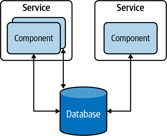
Figure 4-3. Centralized data management in a traditional data-centric application

This approach has several advantages; for instance, the data in these database tables can be normalized, providing high data consistency. Furthermore, as components can access all the tables, the centralized data storage provides the ability to run stored procedures across multiple tables and to retrieve results faster. On the other hand, this provides tight coupling between applications, and hinders the ability to evolve the applications independently. Therefore, it is considered an antipattern when building cloud native applications.

Decentralized Data Management

To overcome problems with centralized data management, each independent functional component can be modeled as a microservice that has separate data stores, exclusive to each of them. This decentralized data management approach, illustrated in Figure 4-4, allows us to scale microservices independently without impacting other microservices.

These databases do not introduce the coupling that can make change riskier and more difficult. Although application owners have less freedom to manage or evolve the data, segregating it in each microservice so that it’s managed by its teams/owners not only solves data management and ownership problems, but also improves the development time of new feature implementations and release cycles.

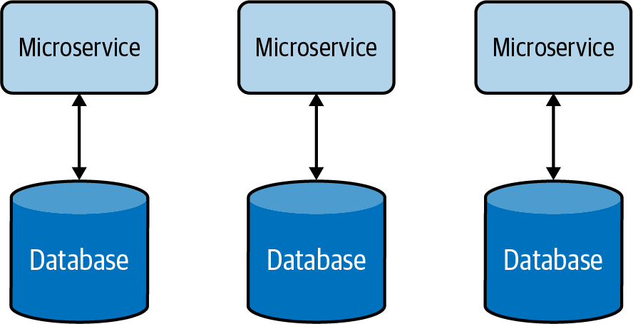
Figure 4-4. Decentralized data management

Decentralized data management allows services to choose the most appropriate data store for their use case. For example, a Payment service may use a relational database to perform transactions, while an Inquiry service may use a document store to store the details of the inquiry, and a Shopping Cart service may use a distributed key-value store to store the items picked by the customer.

Hybrid Data Management

Apart from the benefits of using a single database that we discussed in the preceding section, there are other operational advantages it can provide. For example, it helps achieve compliance with modern data-protection laws and ease security enforcement as data resides in a central place. Therefore, it is advisable to have all customer data managed via a few microservices within a secured bounded context, and to provide ownership of the data to one or a few well-trained teams to apply data-protection policies.

On the other hand, one of the disadvantages of decentralized data management is the cost of running separate data stores for each service. Therefore, for some small and medium organizations, we can use a hybrid data management approach (Figure 4-5). This allows multiple microservices to share the same database, provided these services are governed by the same team and reside in the same bounded context.

But when using hybrid data management, we have to make sure that our services do not directly access tables owned by other services. Otherwise, this will increase the system’s complexity and make it difficult to separate data into multiple databases in the future.

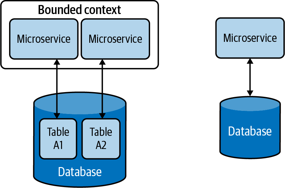
Figure 4-5. Hybrid data management

Data Management Summary

In this section, we looked at how cloud native applications are modeled as independent microservices, and how we achieve scalability, maintainability, and security, by exclusively using separate data stores for each microservice (Figure 4-6).

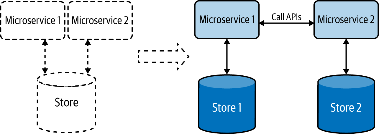
Figure 4-6. Cloud native applications, depicted at right, have a dedicated data store for each microservice.

We’ve seen how applications communicate with each other via well-defined APIs, and we can use this approach to retrieve data from respective applications without accessing their data stores directly.

Now that we’ve covered the types and formats of data, as well as storage and management options, let’s dig into the data-related patterns that we can apply when developing our cloud native applications. The data management patterns provide a good way to understand how to better handle data with respect to data composition, scalability, performance optimization, reliability, and security. Relevant data management patterns are discussed in detail next, including their usage, real-world use cases, considerations, and related patterns.

Data Composition Patterns

This section describes ways in which data can be shared and combined in a meaningful way that helps you efficiently build cloud native applications. Let’s consider a simple cloud native application and its data store, shown in Figure 4-7. Here the application’s microservice fully owns the data residing in its data store.

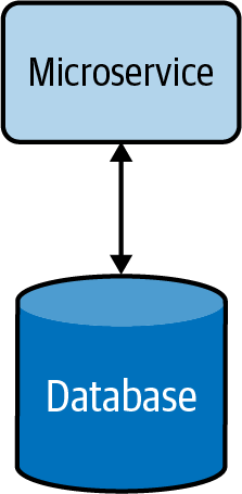
Figure 4-7. Basic cloud native microservice

When the service is under high load, it can introduce high latency due to longer data-retrieval time. This can be mitigated by using a cache (Figure 4-8). This reduces the load on the database when multiple read requests occur and improves the overall performance of the service. More information on caching patterns and other performance optimization techniques are discussed in detail later in this chapter.

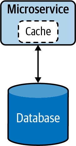
Figure 4-8. Cloud native microservice with cache

When the functionality of the service becomes more complex, the service can be split into smaller microservices (Figure 4-9). During this phase, relevant data will also be split and moved along with the new services, as having multiple services share the same data is not recommended.

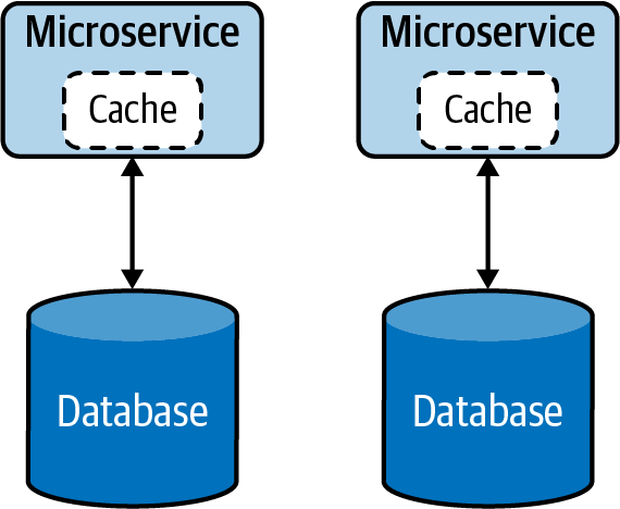
Figure 4-9. Segregation of microservice by functionality

At times, splitting the data in two might not be straightforward, and we might need an alternative option for sharing data in a safe and reusable manner. The following Data Service pattern explains in detail how this can be handled.

Data Service Pattern

The Data Service pattern exposes data in the database as a service, referred to as a data service. The data service becomes the owner, responsible for adding and removing data from the data store. The service may perform simple lookups or even encapsulate complex operations when constructing responses for data requests.

How it works

Exposing data as a data service, shown in Figure 4-10, provides us more control over that data. This allows us to present data in various compositions to various clients, apply security, and enforce priority-based throttling, allowing only critical services to access data during resource-constraint situations such as load spikes or system failures.

These data services can perform simple read and write operations to a database or even perform complex logic such as joining multiple tables or running stored procedures to build responses much more efficiently. These data services can also utilize caching to enhance their read performance.

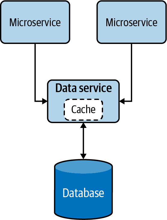
Figure 4-10. Data Service pattern

How it’s used in practice

This pattern can be used when we need to allow access to data that does not belong to a single microservice, or when we need to abstract legacy/proprietary data stores to other cloud native applications.

Allow multiple microservices to access the same data

We can use this pattern when the data does not belong to any particular microservice; no microservice is the rightful owner of that data, yet multiple microservices are depending on it for their operation. In such cases, the common data should be exposed as an independent data service, allowing all dependent applications to access the data via APIs.

For example, say an ecommerce system has Order and Product Detail microservices that need to access discount data. Because the discount does not belong to either of those microservices, a separate service should be created to expose discount data. Now, both Order and Product Detail microservices should access the new discount data service via APIs for information.

Expose abstract legacy/proprietary data stores

We can also use this pattern to expose legacy on-premises or proprietary data stores to other cloud native applications. Let’s imagine that we have a legacy database to record all business transactions for our proprietary on-premises application. In this case, if we need our cloud native applications to access that data, we need to use its C# database driver and make sure all of them know the table and structure of the database to access the data.

It might be not a good idea to access the database directly through the driver, as this will force us to write all our cloud native applications in C#, and all our applications should also embed the knowledge of the table. Instead, we can create a single data service that fronts the legacy database and exposes that data via well-defined APIs. This will allow other cloud native applications to access the data via APIs and decouple themselves from the underlying database table and programming language. This will also allow us to migrate the database to a different one in the future without affecting services that are depending on the data service.

Considerations

When building cloud native applications, accessing the same data via multiple microservices is considered an antipattern. This will introduce tight coupling between the microservices and not allow the microservices to scale and evolve on their own. The Data Service pattern can help reduce coupling by providing managed APIs to access data.

This pattern should not be used when the data can clearly be associated with an existing microservice, as introducing unnecessary microservices will cause additional management complexity.

Related patterns

The following patterns, all covered in this chapter, are related to the Data Service pattern:

Caching pattern

Provides an opportunity to optimize the efficiency of data retrieval by using local or distributed caching when exposing data via a service.

Performance optimization patterns

Apart from caching data, these execute complex queries such as table joins and running stored procedures directly in the database to improve performance.

Materialized View pattern

Accessing data via an API can still be performance-intensive. For use cases that need joins to be performed with data that resides in stores belonging to other services, having that data replicated in its local store and building a materialized view can help improve query performance.

Vault Key pattern

Along with API security, knowing who is accessing the data can help identify the caller and enforce adequate security and data protection.

Composite Data Services Pattern

The Composite Data Services pattern performs data composition by combining data from more than one data service and, when needed, performs fairly complex aggregation to provide a richer and more concise response. This pattern is also called the Server-Side Mashup pattern, as data composition happens at the service and not at the data consumer.

How it works

This pattern, which resembles the Service Orchestration pattern from Chapter 3, combines data from various services and its own data store into one composite data service. This pattern not only eliminates the need for multiple microservices to perform data composition operations, but also allows the combined data to be cached for improving performance (Figure 4-11).

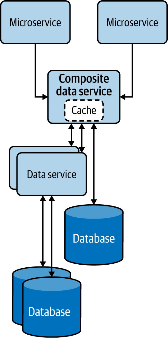
Figure 4-11. Composite Data Services pattern

How it’s used in practice

This pattern can be used when we need to eliminate multiple microservices repeating the same data composition. Data services that are fine-grained force clients to query multiple services to build their desired data. We can use this pattern to reduce duplicate work done by the clients and consolidate it into a common service.

Let’s take an ecommerce system that calculates product inventory by aggregating various data services exposed by different fulfillment stores. In this case, introducing a common service to combine data from all fulfillment services can be beneficial, as this will help remove the duplicate work, reduce the complexity of each client, and help the composite data services evolve without hindering the clients.

When such data is cached at the composite data service, the response time for inventory information can also be improved. This is because, in a given time frame, most of the microservices will be accessing the same set of data, and caching can drastically improve their read performance.

Considerations

Use this pattern only when the consolidation is generic enough and other microservices will be able to reuse the consolidated data. We do not recommend introducing unnecessary layers of services if they do not provide meaningful data compositions that can be reused. Weigh the benefits of reusability and simplicity of the clients against the additional latency and management complexity added by the service layers.

Related patterns

The Composite Data Services pattern is related to the following (both covered in this chapter):

Caching pattern

Provides an opportunity to optimize the efficiency of data retrieval and helps achieve resiliency by serving data from the cache when backends are not available.

Client-Side Mashup pattern

Allows the data mashup to happen at the client side, such as in the user’s browser. This can be a good solution when asynchronous data loading is feasible and when meaningful data composition can be performed with partial data.

Client-Side Mashup Pattern

In the Client-Side Mashup pattern, data is retrieved from various services and consolidated at the client side. The client is usually a browser loading data via asynchronous Ajax calls.

How it works

This pattern utilizes asynchronous data loading, as shown in Figure 4-12. For example, when a browser using this pattern is loading a web page, it loads and renders part of the web page first, while loading the rest of the web page. This pattern uses client-side scripts such as JavaScript to asynchronously load the content in the web browser.

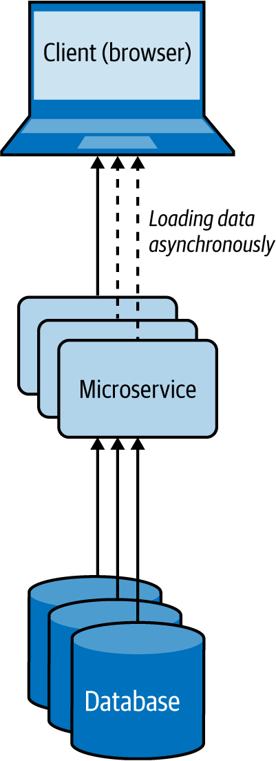
Figure 4-12. Client-Side Mashup at a web browser

Rather than letting the user wait for a longer time by loading all content on the website at once, this pattern uses multiple asynchronous calls to fetch different parts of the website and renders each fragment when it arrives. These applications are also referred to as rich internet applications (RIAs).

How it’s used in practice

This pattern can be used when we need to present available data as soon as possible, while providing more detail later, or when we want to give a perception that the web page is loading much faster.

Present critical data with low latency

Let’s take a use case of an ecommerce system like Amazon; when the user loads a product detail page, we should be able to present all the critical data that the user expects, with the lowest latency. Getting these product reviews and loading images can take time, so we render the page with basic product details with the default image, and then use Ajax calls to load other product images and reviews, and update the web page dynamically. This approach will allow us to deliver the most critical data to the user much faster than waiting for all data to be fetched.

Give a perception that the web page is loading faster

If we are retrieving loosely related HTML content and building the web page while the user is loading it, and if we can allow the user to view part of the content while the rest is being loaded, then we can give the perception that the web site is loading faster. This keeps the user engaged with the website until the rest of the data is available and can ultimately improve the user experience.

Considerations

Use this pattern only when the partial data loaded first can be presented to the user or used in a meaningful way. We do not advise using this pattern when the retrieved data needs to be combined and transformed with later data via some sort of a join before it can be presented to the user.

Related patterns

The Client-Side Mashup pattern is related to the following patterns (covered in this chapter):

Composite Data Services pattern

This is useful when content needs to be mashed synchronously and the composite data is common enough to be used by multiple services.

Caching pattern

Provides an opportunity to cache data to improve the overall latency.

Summary of Data Composition Patterns

This section outlined commonly used patterns of data composition in cloud native application development. Table 4-2 summarizes when we should and should not use these patterns and the benefits of each.

Table 4-2. Data composition patterns

Pattern	When to use	When not to use	Benefits
Data Service	Data is not owned by a single microservice, yet multiple microservices are depending on the data for their operation.	Data can clearly be associated with an existing microservice, as introducing unnecessary microservices can also cause management complexity.	Reduces the coupling between services. Provides more control/security on the operations that can be performed on the shared data.
Composite Data Services	Many clients query multiple services to consolidate their desired data, and this consolidation is generic enough to be reused among the clients.	Only one client needs the consolidation. Operations performed by clients cannot be generalized to be reused by many clients.	Reduces duplicate work done by the clients and consolidates it into a common service. Provides more data resiliency by using caches or static data.
Client-Side Mashup	Some meaningful operations can be performed with partial data; for example, rendering nondependent data in web browsers.	Processing, such as a join, is required on the independently retrieved data before sending the response.	Results in more-responsive applications. Reduces the wait time.

Data Scaling Patterns

When load increases in cloud native applications, either the service or the store can become a bottleneck. The patterns for scaling services are discussed in Chapter 3. Here, we will see how to scale data. When the data can be categorized as big data, we can use NoSQL databases or distributed filesystems. These systems do the heavy lifting of scaling and partitioning the data and reduce the development and management complexity.

Nevertheless, consistency and transactional requirements of business-critical applications may still require us to use relational databases, and as relational databases do not scale by default, we might need to alter the application architecture to achieve data scalability. In this section, we’ll dive deep into the patterns that can help us facilitate the scaling of data stores to optimally store and retrieve data.

Data Sharding Pattern

In the Data Sharding pattern, the data store is divided into shards, which allows it to be easily stored and retrieved at scale. The data is partitioned by one or more of its attributes so we can easily identify the shard in which it resides.

How it works

To shard the data, we can use horizontal, vertical, or functional approaches. Let’s look at these three options in detail:

Horizontal data sharding

Each shard has the same schema, but contains distinct data records based on its sharding key. A table in a database is split across multiple nodes based on these sharding keys. For example, user orders can be shared by hashing the order ID into three shards, as depicted in Figure 4-13.

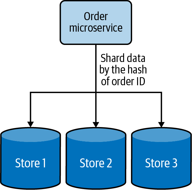
Figure 4-13. Horizontal data sharding using hashing

Vertical data sharding

Each shard does not need to have an identical schema and can contain various data fields. Each shard can contain a set of tables that do not need to be in another shard. This is useful when we need to partition the data based on the frequency of data access; we can put the most frequently accessed data in one shard and move the rest into a different shard. Figure 4-14 depicts how frequently accessed user data is sharded from the other data.

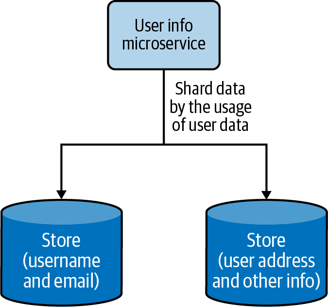
Figure 4-14. Vertical data sharding based on frequency of data access

Functional data sharding

Data is partitioned by functional use cases. Rather than keeping all the data together, the data can be segregated in different shards based on different functionalities. This also aligns with the process of segregating functions into separate functional services in the cloud native application architecture. Figure 4-15 shows how product details and reviews are sharded into two data stores.

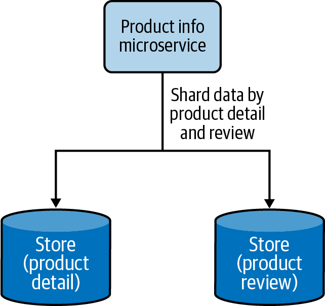
Figure 4-15. Functional data sharding by segregating product details and reviews into two data stores

Cloud native applications can use all three approaches to scale data, but there is a limit to how much the vertical and functional sharding can segregate the data. Eventually, horizontal data sharding needs to be brought in to scale the data further. When we use horizontal data sharding, we can deploy one of the following techniques to locate where we have stored the data:

Lookup-based data sharding

A lookup service or distributed cache is used to store the mapping of the shard key and the actual location of the physical data. When retrieving the data, the client application will first check the lookup service to resolve the actual physical location for the intended shard key, and then access the data from that location. If the data gets rebalanced or resharded later, the client has to again look up the updated data location.

Range-based data sharding

This special type of sharding approach can be applied when the sharding key has sequential characters. The data is shared in ranges, and as in lookup-based sharding, a lookup service can be used to determine where the given data range is available. This approach yields the best results for sharding keys based on date and time. A data range of a month, for example, may reside in the same shard, allowing the service to retrieve all the data in one go, rather than querying multiple shards.

Hash-based data sharding

Constructing a shard key based on the data fields or dividing the data by date range may not always result in balanced shards. At times we need to distribute the data randomly to generate better-balanced shards. This can be done by using hash-based data sharding, which creates hashes based on the shard key and uses them to determine the shard data location. This approach is not the best when data is queried in ranges, but is ideal when individual records are queried. Here, we can also use a lookup service to store the hash key and the shard location mapping, to facilitate data loading.

For sharding to be useful, the data should contain one or a collection of fields that uniquely identifies the data or meaningfully groups it into subsets. The combination of these fields generates the shard/partition key that will be used to locate the data. The values stored in the fields that contribute to the shard key should be fixed and never be changed upon data updates. This is because when they change, they will also change the shard key, and if the updated shard key now points to a different shard location, the data also needs to be migrated from the current shard to the new shard location. Moving data among shards is time-consuming, so this should be avoided at all costs.

How it’s used in practice

This pattern can be used when we can no longer store data in a single node, or when we need data to be distributed so we can access it with lower latency.

Scale beyond a single node

This pattern can be useful when resources such as storage, computation, or network bandwidth become a bottleneck. A system’s ability to vertically scale is always limited when adding more resources such as disk space, RAM, or network bandwidth; sooner or later, the application will run out of resources. Instead of working on short-term solutions, partitioning the data and scaling horizontally will help you scale beyond the capacity of a single node.

Segregate data to improve data-retrieval time

We can segregate data by combining multiple data fields to generate special shard keys. For example, let’s imagine we have an online fashion store and have created a shard key that combines a dress type and brand in order to store data. If we know the type and brand of the dress that we are searching for, we will be able to map that to the relevant shard and quickly retrieve the data. But if we know only the type and size of the dress, we cannot construct a valid shard key. In this case, we need to search all shards to find the match, and this can greatly impact our performance.

This problem can be overcome by building hierarchical shard keys. For example, we can build the key with the dress type / brand. If we know the dress type, we can look up all shards that have that dress type and then search them for the particular dress size. This restricts the number of shards that we need to search and improves performance. If we need even better performance for the type and size combination, we can create secondary indexes using them. These secondary shard keys can help us retrieve the data with low latency. But the use of secondary indexes can increase the data modification cost, as now we also need to update the secondary shard keys when data is updated.

We can also shard the data by date and time ranges. For example, if we are processing orders, we are likely more interested in recent orders than old ones. We can shard data by time ranges and store the most recent orders (such as last-month or last-quarter orders) in a hot shard and the rest in a set of archived shards. This can help retrieve the critical data with efficiency. In this case, we should also periodically move the data from the hot shard to archive shards when it becomes old.

Geographically distribute data

When the clients are geographically distributed, we can shard the data by region and move the relevant data closer to them. For example, in a retail website use case, details about products sold in each region can be stored and served locally. This will help serve more requests at a lower turnaround time.

Some clients may be interested in buying products from around the world, so we might need to retrieve data from multiple shards distributed across regions to fulfill a request. For this use case to work efficiently, we need to model the clients in such a way that they can issue a fan-out request to all the shards and retrieve data concurrently. For example if a user is searching the products, we can send a fan-out request and just respond with the first 10 fastest entries we receive, but if the user is searching for the lowest-price options by name, we might need to wait for the response to arrive from all shards before showing the results. Note that we might be able to improve the performance with caching. We discuss that later in this chapter.

Considerations

When we use this pattern, it is important to balance the shards as much as possible in order for the load to distribute evenly. It is also necessary to monitor the load in each shard and perform a rebalance if the load is not distributed evenly. Imbalance can happen over time, due to new data skew with insertions, deletions, or a change in querying behavior. Keep in mind that with big data, rebalancing of data stores can take a couple of hours to days.

To facilitate rebalancing, we recommend making the shards reasonably smaller. In the initial days of the system, when the data and load are low, all shards can live in the same node. Eventually, when load increases, one or a collection of shards can be migrated to other nodes. This not only allows greater scalability in the long run, but also makes each shard migration relatively small, allowing the data rebalancing to happen faster with less interruption to the whole system.

It is also important to have multiple copies of shards to gracefully handle failures. Even when a node is down, we will have access to the same data in another node, and this can help us perform maintenance without making the full system unavailable.

When it comes to processing data aggregation across shards, different aggregations behave differently. Aggregations such as sum, average, minimum, and maximum can process the data in isolation at each partition, retrieve the results, and combine them to determine the final results. In contrast, aggregation operations such as median require the whole data at once, so this cannot be implemented with high precision when using sharded data.

We don’t recommend using auto-incrementing fields when generating shard keys. Shards do not communicate with each other, and because of the use of auto-incrementing fields, multiple shards may have generated the same keys and refer to different data with those keys locally. This can become a problem when the data is redistributed during data-rebalancing operations.

Furthermore, it is important to select shard keys that will result in fairly balanced shards. Without balanced shards, the expected scalability cannot be achieved. The largest shard is always going to be the worst-performing one and will eventually cause bottlenecks.

Related patterns

The Data Sharding pattern is related to the following (both covered in this chapter):

Materialized View pattern

This can be used to replicate the dependent data of each shard to the local stores of the service, to improve data-querying performance and eliminate multiple lookup calls to data stores or services. This data can be replicated with only eventual consistency, so this approach is useful only if consistency on the dependent data is not business-critical for the applications.

Data Locality pattern

Having all the relevant data at the shard will allow the creation of indexes and execution of stored procedures for efficient data retrieval.

Command and Query Responsibility Segregation Pattern

The Command and Query Responsibility Segregation (CQRS) pattern separates updates and query operations of a data set, and allows them to run on different data stores. This results in faster data update and retrieval. It also facilitates modeling data to handle multiple use cases, achieves high scalability and security, and allows update and query models to evolve independently with minimal interactions.

How it works

We can separate commands (updates/writes) and queries (reads) by creating different services responsible for each (Figure 4-16). This not only facilitates running services related to update and reads on different nodes, but also helps model services appropriate for those operations and independently scale the services.

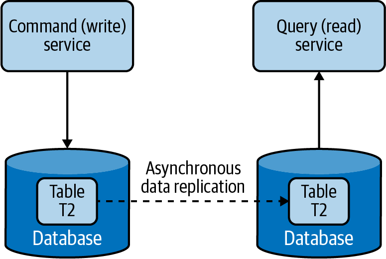
Figure 4-16. Separating command and query operations

The command and query should not have data store–specific information but rather have high-level data relevant to the application. When a command is issued to a service, it extracts the information from the message and updates the data store. Then it will send that information as an event asynchronously to the services that serve the queries, such that they can build their data model. The Event Sourcing pattern using a log-based queue system like Kafka can be used to pass the events between services. Through this, the query services can read data from the event queues and perform bulk updates on their local stores, in the optimal format for serving that data.

How it’s used in practice

We can use this pattern when we want to use different domain models for commands and queries, and when we need to separate updates and data retrieval for performance and security reasons. Let’s look at these approaches in detail next.

Use different domain models for command and query

For a retail website, we may be storing the product detail and inventory information in a normalized relational database. This might be our best choice to efficiently update inventory information upon each purchase. But this may not be the best option for querying this data via a browser, as joining and converting the data to JSON can be time-consuming. If that is the case, we can use this pattern to asynchronously build a query data set, such as a document store storing data in JSON format, and use that for querying. Then we will have separate optimized data models for both command and query operations.

Because command and query models are not tightly coupled, we can use different teams to own command- and query-related applications, as well as allow both models to evolve independently according to the use case.

Distribute operations and reduce data contention

This pattern can be used when cloud native applications have performance-intensive update operations such as data and security validations, or message transformations, or have performance-intensive query operations containing complex joins or data mapping. When the same instance of the data store is used for both command and query, it can produce poor overall performance due to higher load on the data store. Therefore, by splitting the command and query operations, CQRS not only eliminates the impact of one on the other by improving the performance and scalability of the system, but also helps isolate operations that need higher security enforcement.

Because this pattern allows commands and queries to be executed in different stores, it also enables the command and query systems to have different scaling requirements. In the retail website use case, we have more queries than commands, and have more product detail views than actual purchases. Hence, we can have most services support query operations and a couple of services perform the updates.

Considerations

Because this pattern segregates the command and query operations, it can provide high availability. Even if some command or query services become unavailable, the full system will not be halted. In this pattern, we can scale the query operations infinitely, and with an appropriate number of replications, the query operations can provide guarantees of zero downtime. When scaling command operations, we might need to use patterns such as Data Sharding to partition data and eliminate potential merge conflicts.

CQRS is not recommended when high consistency is required between command and query operations. When data is updated, the updates are sent asynchronously to the query stores via events by using patterns such as Event Sourcing. Hence, use CQRS only when eventual consistency is tolerable. Achieving high consistency with synchronous data replication is not recommended in cloud native application environments as it can cause lock contention and introduce high latencies.

When using this pattern, we may not be able to automatically generate separate command and query models by using tools such as object-relational mapping (ORM). Most of these tools use database schemas and usually produce combined models, so we may need to manually modify the models or write them from scratch.

Note

Though this pattern looks fascinating, remember that it can introduce lots of complexity to the system architecture. We now need to keep various data sources updated by sending events via the Event Sourcing pattern, as well as handle event duplicates and failures. Therefore, if the command and query models are quite simple, and the business logic is not complex, we strongly advise you to not use this pattern. It can introduce more management complexity than the advantages it can produce.

Related patterns

The following are related to CQRS:

Event Sourcing pattern

Allows command services to communicate updates to query services, and allows both command and query models to reside on different data stores. This provides only eventual consistency between command and query models and adds complexity to the system architecture. Chapter 5 covers this pattern in detail.

Materialized View pattern

Recommended over the CQRS pattern to achieve scalability, when command and query models are simple enough; Materialized View is covered in the next section.

Data Sharding pattern

Helps scale commands by partitioning the data (as covered previously in this chapter). As query operations can simply be replicated, applying this pattern for queries may not produce any performance benefit.

API security

Can be applied to enforce security for both command and query services.

Summary of Data Scaling Patterns

This section outlined commonly used patterns of data scaling in cloud native application development. Table 4-3 summarizes when we should and should not use these patterns and the benefits of each.

Table 4-3. Data scaling patterns

Pattern	When to use	When not to use	Benefits
Data Sharding	Data contains one or a collection of fields that uniquely identify the data or meaningfully group the data into subsets.	Shard key cannot produce evenly balanced shards. The operations performed in the data require the whole set of data to be processed; for example, obtaining a median from the data set.	Groups shards based on the preferred set of fields that produce the shard key. Creates geographically optimized shards that can be moved closer to the clients. Builds hierarchical shards or time-range-based shards to optimize the search time. Uses secondary indexes to query data by using nonshard keys.
Command and Query Responsibility Segregation (CQRS)	Applications have performance-intensive update operations with: Data validations Security validations Message transformations For performance-intensive query operations such as complex joins or data mapping.	High consistency is required between command (update) and query (read). Command and query models are closer to each other.	Reduces the impact between command and query operations. Stores command and query data in two different data stores that suit their use cases. Enforces separated command/query security policies. Enables different teams to own applications that are responsible for command and query operations. Provides high availability.

Performance Optimization Patterns

In distributed cloud native applications, data is often the most common cause of bottlenecks. Data is difficult to scale, as consistency requirements can cause lock contention and synchronization overhead. All of this results in systems that perform poorly.

One primitive way of improving performance is by indexing data. Though this improves lookup performance, overuse of indexes can impair both read and write performance. For every write operation, all indexes need to be updated, causing databases to perform multiple writes. Similarly, when it comes to reads, data stores might not be able to load all indexes and keep them in memory. Each query might need to perform a couple of read operations, resulting in more time to fetch data.

Data denormalization is also a good technique for simplifying read models, as it can eliminate the need for joins and drastically improve read performance. This can be especially useful when we combine this approach with the CQRS pattern, as writers can use normalized data stores to maintain high consistency while allowing queries to read from denormalized data with efficiency.

In addition to these simple techniques, let’s discuss how to improve performance by moving data closer to the execution, moving execution closer to the data, reducing the amount of data being transferred, or by storing preprocessed data for future use. This section discusses such patterns in detail.

Materialized View Pattern

The Materialized View pattern provides the ability to retrieve data efficiently upon querying, by moving data closer to the execution and prepopulating materialized views. This pattern stores all relevant data of a service in its local data store and formats the data optimally to serve the queries, rather than letting that service call dependent services for data when required.

How it works

This pattern replicates and moves data from dependent services to its local data store and builds materialized views (Figure 4-17). It also builds optimal views to efficiently query the data, similar to the Composite Data Services pattern.

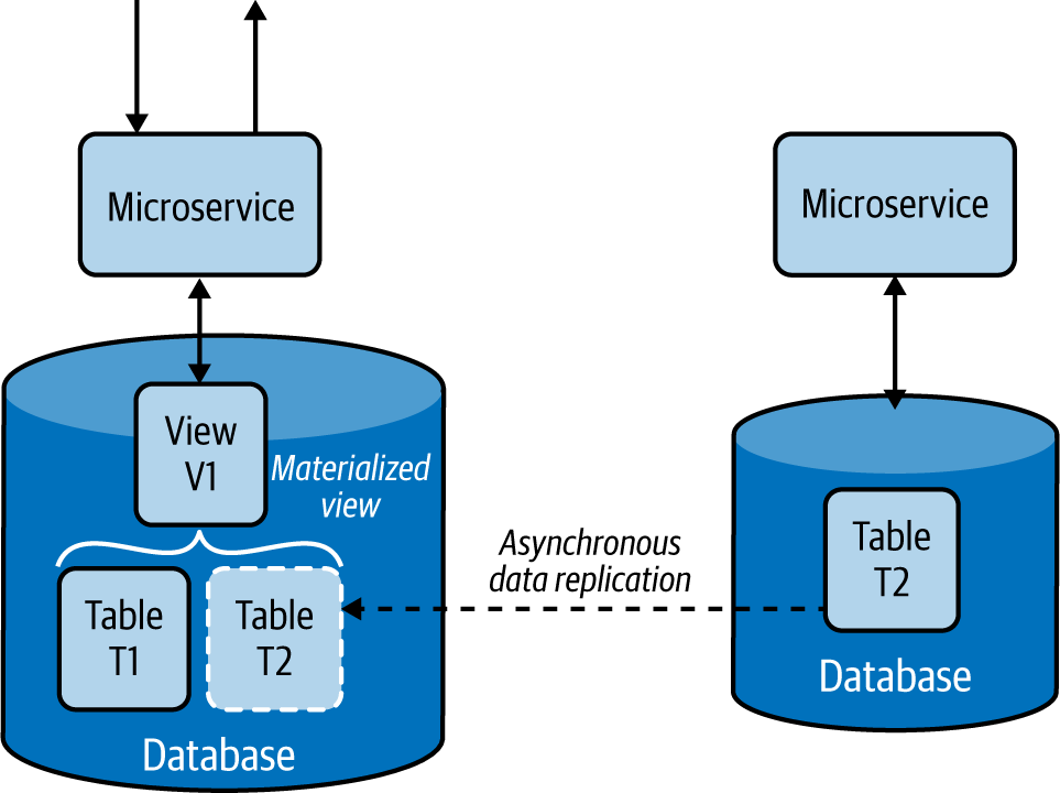
Figure 4-17. Service built with the Materialized View pattern

This pattern asynchronously replicates data from the dependent services. If databases support asynchronous data replication, we can use it as a way to transfer data from one data store to another. Failing this, we need to use the Event Sourcing pattern and use event streams to replicate the data. The source service pushes each insert, delete, and update operation asynchronously to an event stream, and they get propagated to the services that build materialized views, where they will fetch and load the data to their local stores. Chapter 5 discusses the Event Sourcing pattern in detail.

How it’s used in practice

We can use this pattern when we want to improve data-retrieval efficiency by eliminating complex joins and to reduce coupling with dependent services.

Improve data-retrieval efficiency

This pattern is used when part of the data is available locally and the rest needs to be fetched from external sources that incur high latency. For example, if we are serving a product detail page of an ecommerce application that, indeed, retrieves comments and ratings from a relatively slow review service, we might be rendering the data to the user with high latency. Through this pattern, the overall rating and precalculated best and worst comments can be replicated to the product detail service’s data store to improve data-retrieval efficiency.

Even when we bring data into the same database, at times joining multiple tables can still be costly. In this case, we can use techniques like relational database views to consolidate data into an easily queryable materialized view. Then, when we need to retrieve product details, the detail service can serve the data with high efficiency.

Provide access to nonsensitive data hosted in secure systems

In some use cases, our caller service might depend on nonsensitive data that is behind a security layer, requiring the service needs to authenticate and go through validation checks before retrieving the data. But through this pattern, we can replicate the nonsensitive data relevant to the service and allow the caller service to access the data directly from its local store. This approach not only removes unnecessary security checks and validations but also improves performance.

Considerations

Sometimes the dependent data may be stored in different types of data stores, or those stores can contain lots of unnecessary data. In this case, we should replicate only the relevant subset of data and store it in a format that can help build the materialized view. This will improve overall query performance by using data locally, and reduce bandwidth usage when transferring the data. We should always use asynchronous data replication, as synchronous data replication can cause lock contention and introduce high latencies.

The Materialized View pattern not only improves service performance by reducing the time to retrieve data, but also simplifies the service logic by eliminating unnecessary data processing and the need to know about dependent services.

This pattern also provides resiliency. As the data is replicated to the local store, the service will be able to perform its operations without any interruption, even when the source service that provided the data is unavailable.

We do not recommend using this pattern when data can be retrieved from dependent services with low latency, when data in the dependent services is changing quickly, or when the consistency of the data is considered important for the response. In these cases, this pattern can introduce unnecessary overhead and inconsistent behavior.

This pattern is not ideal when the amount of data that needs to be moved is huge or the data is updated frequently. This can cause replication delays and high network bandwidth, affecting accuracy and performance of the application. Consider using the Data Locality pattern (covered next) for these use cases.

Related patterns

The following are related to the Material View pattern; all but the last are covered in this chapter:

Data Locality pattern

Enables efficient data retrieval by moving the execution closer to the data.

Composite Data Services pattern

This can be used instead of the Materialized View pattern when data compositions can be done at the service level, or when dependent services have static data that can be cached locally at the service.

Command and Query Responsibility Segregation (CQRS) pattern

The Materialized View pattern can be used to serve query responses in the CQRS pattern. The command—the modifications to the data—will be done through the dependent service, and the query—the serving of the read requests—can be performed by query services constructing the materialized views.

Event Sourcing pattern

Provides an approach to replicate data from one source to another. Changes on dependent data are pushed as events through event streams, which are stored sequentially at a reliable log-based event queue such as Kafka, and then the services that serve the data read those event streams and constantly update their local storage to serve updated information. Chapter 5 covers this pattern.

Data Locality Pattern

The goal of the Data Locality pattern is to move execution closer to the data. This is done by colocating the services with the data or by performing the execution in the data store itself. This allows the execution to access data with fewer limitations, helping to quicken execution, and to reduce bandwidth by sending aggregated results.

How it works

Moving execution can improve performance more than moving data. When enough CPU resources are available, adding a service dedicated to the query at the data node, as shown in Figure 4-18, can improve performance by processing most of the data locally rather than transferring it over the network.

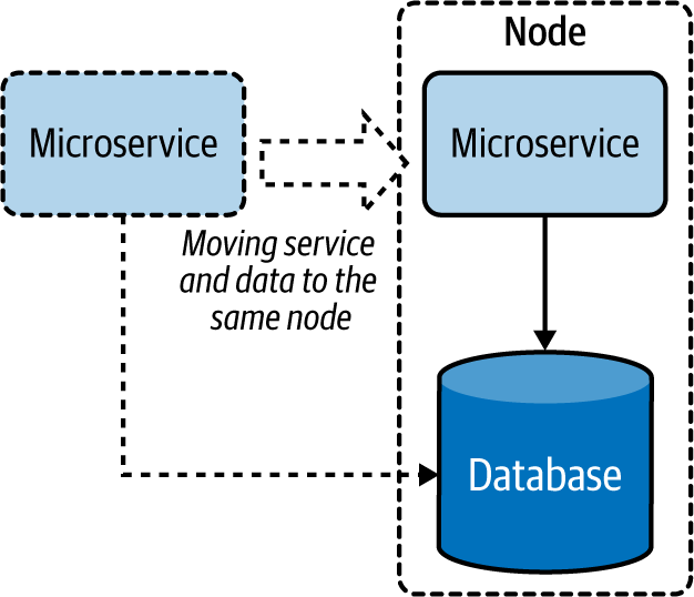
Figure 4-18. Moving a microservice closer to the data store

When the service cannot be moved to the same node, moving the service to the same region or data center can help better utilize the bandwidth. This approach can also help the service cache results and serve from them more efficiently.

We can also move execution closer to the data by moving it to the data store as stored procedures (Figure 4-19). This is a great way to utilize the capabilities of relational databases to optimize data processing and retrieval.

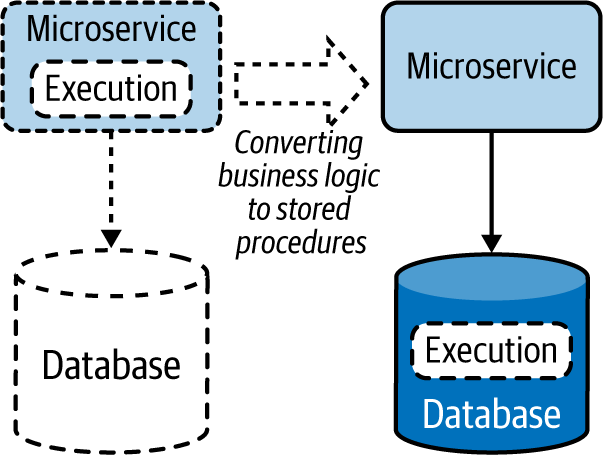
Figure 4-19. Moving execution to data stores as stored procedures

How it’s used in practice

This pattern encourages coupling execution with data to reduce latency and save bandwidth, enabling distributed cloud native applications to operate efficiently over the network.

Reduce latency when retrieving data

We can use this pattern when we need to retrieve data from one or more data sources and perform some sort of join. To process data, a service needs to fetch all the data to its local memory before it can perform a meaningful operation. This requires data to be transferred over the network, introducing latency. By moving the service closer to the data store (or when there are multiple stores involved, moving it to the store that contributes to the most input) will reduce data being transferred via the network, thus reducing data-retrieval time. We can also use this pattern for composition services that perform joins by consuming data from data stores and other services. By moving these services closer to the data source, we can improve their overall performance.

Reduce bandwidth usage when retrieving data

This pattern is especially useful when we need to retrieve data from multiple sources to perform data aggregation or filtering operations. The output of these queries will be significantly smaller than their input. By running the execution closer to the data source, we need to transfer only a small amount of data, which can improve bandwidth utilization. This is especially useful when data stores are huge and clients are geographically distributed. This is a good approach when cloud native applications are experiencing bandwidth bottlenecks.

Considerations

Applying the Data Locality pattern can also help utilize idle CPU resources at the data nodes. Most data nodes are I/O intensive, and when the queries they perform are simple enough, they might have plenty of CPU resources idling. Moving execution to the data node can better utilize resources and optimize overall performance. We should be careful to not move all executions to the data nodes, as this can overload them and cause issues with data retrieval.

This pattern is not ideal when queries output most of their input. These cases will overload the data nodes without any savings to bandwidth or performance. Deciding when to use this pattern depends on the trade-off between bandwidth and CPU utilization. We recommend using this pattern when the gains achieved by reducing the data transfer are much greater than the additional execution cost incurred at the data nodes.

Note

Transfer the execution to the data store only when that data store is exclusively used by the querying microservice. Running stored procedures in a shared database is an antipattern, as it can cause performance and management implications. Also be aware that change management of databases is nontrivial, and if not done carefully, the update of the stored procedure could incur downtime. Move execution to the data store only with caution, and prefer having the business logic in the microservice when there is no significant performance improvement.

Related patterns

The following patterns, covered in this chapter, are related to the Data Locality pattern:

Materialized View pattern

Provides an alternative approach for this pattern, by moving data closer to the place of execution. This pattern is ideal when the data is small or when CPU-intensive operations such as complex joins and data transformations are needed during reads.

Caching pattern

Complements this pattern by storing preprocessed data and serving it during repeated queries.

Caching Pattern

The Caching pattern stores previously processed or retrieved data in memory, and serves this data for similar queries issued in the future. This not only reduces repeated data processing at the services, but also eliminates calls to dependent services when the response is already stored in the service.

How it works

A cache is usually an in-memory data store used to store previously processed or retrieved data so we can reuse that data when required without reprocessing or retrieving it again. When a request is made to retrieve data, and we can find the necessary data stored in the cache, we have a cache hit. If the data is not available in the cache, we have a cache miss.

When a cache miss occurs, the system usually needs to process or fetch data from the data store, as well as update the cache with the retrieved data for future reference. This process is called a read-through cache operation. Similarly, when a request is made to update the data, we should update it in the data store and remove or invalidate any relevant previously fetched entries stored in the cache. This process is called a write-through cache operation. Here, invalidation is important, because when that data is requested again, the cache should not return the old data but should retrieve updated data from the store by using the read-through cache operation. This reading and updating behavior is commonly referred to as a cache aside, and most commercial caches support this feature by default.

Caching data can happen on either the client or server side, or both, and the cache itself can be local (storing data in one instance) or shared (storing data in a distributed manner).

Especially when the cache is not shared, it cannot keep on adding data, as it will eventually exhaust available memory. Hence, it uses eviction policies to remove some records to accommodate new ones. The most popular eviction policy is least recently used (LRU), which removes data that is not used for a long period to accommodate new entries. Other policies include first in, first out (FIFO), which removes the oldest loaded entry; most recently used (MRU), which removes the last-used entry; and trigger-based options that remove entries based on values in the trigger event. We should use the eviction policy appropriate for our use case.

When data is cached, data stored in the data store can be updated by other applications, so holding data for a long period in the cache can cause inconsistencies between the data in the cache and the store. This is handled by using an expiry time for each cache entry. This helps reload the data from the data store upon time-out and improves consistency between the cache and data store.

How it’s used in practice

This pattern is usually applied when the same query can be repeatedly called multiple times by one or more clients, especially when we don’t have enough knowledge about what data will be queried next.

Improve time to retrieve data

Caching can be used when retrieving data from the data store requires much more time than retrieving from the cache. This is especially useful when the original store needs to perform complex operations or is deployed in a remote location, and hence the network latency is high.

Improve static content loading

Caching is best for static data or for data that is rarely updated. Especially when the data is static and can be stored in memory, we can load the full data set to the cache and configure the cache not to expire. This drastically improves data-retrieval time and eliminates the need to load the data from the original data source.

Reduce data store contention

Because it reduces the number of calls to the data store, we can use this pattern to reduce data store contention or when the store is overloaded with many concurrent requests. If the application consuming the data can tolerate inconsistencies, such as data being outdated by a few minutes, we can also deploy this pattern on write-intensive data stores to reduce the read load and improve the stability of the system. In this case, the data in the cache will eventually become consistent when the cache times out.

Prefetch data to improve data-retrieval time

We can preload the cache fully or partially when we know the kind of queries that are more likely to be issued. For example, if we are processing orders and know that the applications will mostly call last week’s data, we can preload the cache with last week’s data when we start the service. This can provide better performance than loading data on demand. When preloading is omitted, the service and the data store can encounter high stress, as most of the initial requests will result in a cache miss.

This pattern also can be used when we know what data will be queried next. For example, if a user is searching for products on a retail website, and we are rendering only the first 10 entries, the user likely will request the next 10 entries. Preloading the next 10 entries to the cache can save time when that data is needed.

Achieve high availability by relaxing the data store dependency

Caching can also be used to achieve high availability, especially when the service availability is more important than the consistency of the data. We can handle service calls with cached data even when the backend data store is not available. As shown in Figure 4-20, we can also extend this pattern by making the local cache fall back on a shared or distributed cache, which in turn can fall back to the data store when the data is not present. This pattern can incorporate the Resilient Connectivity pattern with a circuit breaker discussed in Chapter 3 for the fallback calls so that they can retry and gracefully reconnect when the backends become available after a failure.

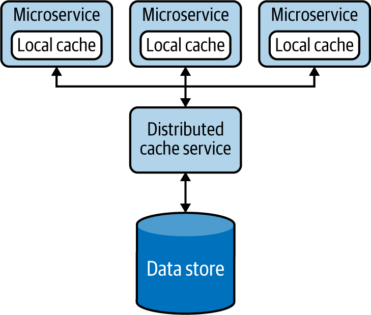
Figure 4-20. Multilayer cache fallback

When using a shared cache, we can also introduce a secondary cache instance as a standby and replicate the data to it, to improve availability. This allows our applications to fall back to the standby when the primary cache fails.

Cache more data than a single node can hold

Distributed caching systems can be used as another alternative option when the local cache or shared cache cannot contain all the needed data. They also provide scalability and resiliency by partitioning and replicating data. These systems support read-through and write-through operations and can make direct calls to the data stores to retrieve and update data. We can also scale them by simply adding more cache servers as needed.

Though distributed caches can store lots of data, they are not as fast as the local cache and add more complexity to the system. We might need additional network hops to retrieve data, and we now need to manage an additional set of nodes. Most important, all nodes participating in the distributed cache should be within the same network and have relatively high bandwidth among one another; otherwise, they can also suffer data-synchronization delays. In contrast, when the clients are geographically distributed, a distributed cache can bring the data closer to the clients, yielding faster response times.

Considerations

The cache should never be used as the single source of truth, and it does not need to be designed with high availability in mind. Even when the caches are not available, the application should be able to execute their expected functionalities. Because caches store data in memory, there is always a possibility of data loss, so data stores are the ones that should be used to persist data for long-term use.

In some cases, most of the data contributing to a response message will be static, and only a small portion of the data will be frequently updated. If constructing the static part of the data is expensive, it may be beneficial to split the records in two, as static and dynamic parts, and then store only those static parts in the cache. When building the response, we can combine the static data stored in the cache and the dynamically generated data.

As an alternative to cache eviction policies, we can also make local caches to support data overflow. This overflow data is written to the disk. You should use this approach only when reading the data from the disk is much faster than retrieving data from the original data store. This approach can introduce additional complexity, as now we also need to manage the cache overflow.

Note

The cache time-out should be set at an optimum level, not too long or too short. While setting a too-long cache time-out can cause higher inconsistencies, setting a too-short time-out is also detrimental, as it will reload the data too often and defeat the purpose of caching data. However, setting a long time-out can also be beneficial when the cost of data retrieval is significantly higher than the cost of data being inconsistent.

The biggest disadvantage of caching data locally is that when services scale, each service will have its own local cache and will sync data with the data stores at different times. One might get an update before the other, and that can lead to a situation where caches in different microservices are not in sync. Then, when the same query is sent to two services, they could respond with different values, because cache invalidation happens only at the service that processes the original update request, and caches in other microservices are not aware of this invalidation. This situation can also occur when the data is replicated at the data store level, as the caches in the microservices are unaware of those updates.

We can mitigate this problem, as shown in Figure 4-21, by invalidating all the caches during data updates by either informing the cache nodes about the update via a messaging system, as in the Publisher-Subscriber pattern, or by using the Event Sourcing pattern. Both patterns are covered in Chapter 5.

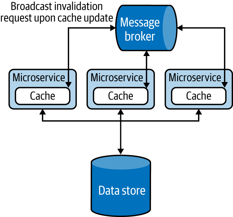
Figure 4-21. Using the message broker to invalidate cache in all services

Note

Introducing unnecessary layers of cache can cause high memory consumption, reduce performance, and cause data inconsistencies. We highly recommend performing a load test when introducing any caching solution, and especially monitoring the percentage of cache hits, along with performance, CPU, and memory usage. A lower cache-hit percentage can indicate that the cache is not effective. In this case, either modify the cache to achieve a higher percentage of cache hits or choose other alternatives. Increasing the size of the cache, reducing cache expiry, and preloading the cache are options that we can use to improve cache hits.

Whenever possible, we recommend batch data updates to caches, as is done in data stores. This optimizes bandwidth and improves performance when the load is high. When multiple cache entries are updated at the same time, the updates can follow either an optimistic or a pessimistic approach. In the optimistic approach, we assume that no concurrent updates will occur and check the cache only for a concurrent write before updating the cache. But in the pessimistic approach, we lock the cache for the full update period so no concurrent updates can occur. The latter approach is not scalable, so you should use this only for very short-lived operations.

We also recommend implementing forceful expiry or reload of the cache. For instance, if the client is aware of a potential update through other means, we can let the client forcefully reload the cache before retrieving data. We can achieve this by introducing a random variable as part of the cache key when storing the data. The client can use the same key over and over again, and change it only when needing to force a reload. This approach is used by web clients against browser caching, for example. Because browsers cache data against a request URI, by having a random element in the URI, the clients can forcefully reload the cached entry by simply changing that random URI element when they are sending the request. Be careful in using this technique with third-party clients because they can continuously change the random variable requesting forceful reload, and overload the system. But if the clients are within the control of the same team, this can be a viable approach.

Some commercial cache services can provide data security by using the Vault Key pattern, covered later in this chapter. But most caches are usually not designed for security, and they should not be directly exposed to external systems. To achieve security, we can add a data service on top of the cache by using the Data Service pattern and apply API security for the data service (Figure 4-22). These will add data protection and allow only authorized services to read and write data to the cache.

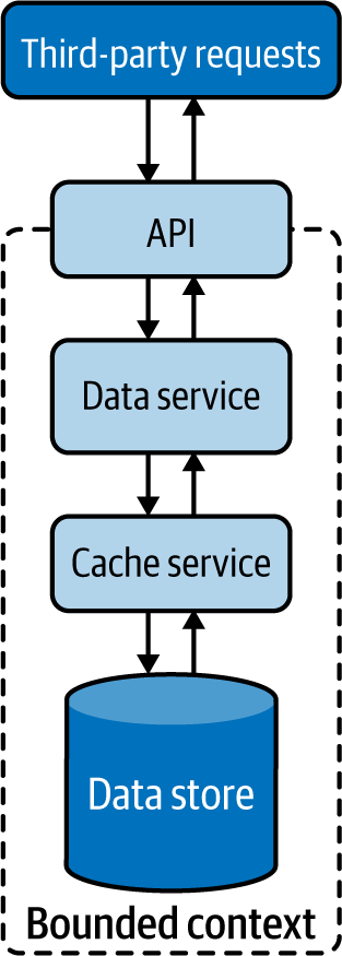
Figure 4-22. Securely exposing the cache to external services

Related patterns

The following patterns (covered in this chapter unless otherwise noted) are related to the Caching pattern:

Data Sharding pattern

Enables the cache to be scaled similarly to the way we can scale data stores. This also enables distributing data geographically so relevant data in the cache can be closer to the services that operate them.

Resilient Connectivity pattern

Provides a mechanism to serve requests from the data sources when data is not available in the cache. Chapter 3 discusses this pattern.

Data Service pattern

Along with API security, can be used to provide a service layer for distributed caches, providing more business-centric APIs for data consumers.

Vault Key pattern

Provides the capability to secure the caches by using access tokens enabling third parties to access the data directly from caches. This can be used only if the caching systems support this functionality. Otherwise, we need to fall back on using the Data Service pattern with API security.

Event Sourcing pattern

Propagates cache-invalidation requests to all local caches. This enables eventual consistency of cache data and reduces the chance of data being obsolete as data sources are updated by multiple services. Chapter 5 details this pattern.

Static Content Hosting Pattern

The Static Content Hosting pattern deploys static content in data stores that are closer to clients so content can be delivered directly to the client with low latency and without consuming excess computational resources.

How it works

Cloud native web services are used to create dynamic content based on clients’ requests. Some clients, especially browsers, require a lot of other static content, such as static HTML pages, JavaScript and CSS files, images, and files for downloads. Rather than using microservices to cater to static content, this pattern allows us to directly serve static content from storage services such as content delivery networks (CDNs).

Figure 4-23 illustrates this pattern in the context of a web application. When the browser requests data, we can make the service respond with dynamic HTML containing embedded links to relevant static data that needs to be rendered at various locations on the page. This allows the browser to then request the static content, which will be resolved by DNS and served from the closest CDN.

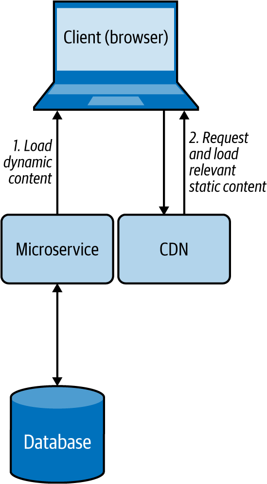
Figure 4-23. Browser loading dynamic content from a microservice while loading static content from a CDN

How it’s used in practice

This pattern is used when we need to quickly deliver static content to clients with low response time, and when we need to reduce the load on rendering services.

Provide faster static content delivery

Because static content does not change, this pattern replicates and caches data in multiple environments and geographical locations with the motivation of moving it closer to the clients. This can help serve static data with low latency.

Reduce resource utilization on rendering services

When we need to send both static and dynamic data to clients, as discussed in the preceding web browser example, we can separate the static data and move it to a storage system such as a CDN or an S3 bucket, and let clients directly fetch that data. This reduces the resource utilization of the microservice that renders the dynamic content, as it does not need to pack all the static content in its response.

Considerations

We cannot use this pattern if the static content needs to be updated before delivering it to the clients, such as adding the current access time and location to the web response. Further, this is not a feasible solution when the amount of static data that needs to be served is small; the cost for the client to request data from multiple sources can incur more latency than is being served directly by the service. When you need to send both static and dynamic content, we recommend using this pattern only when it can provide a significant performance advantage.

When using this pattern, remember that you might need more-complex client implementations. This is because, based on the dynamic data that arrives, the client should be able to retrieve the appropriate static content and combine both types of data at the client side. If we are using this pattern for use cases other than web-page rendering in a browser, we have to also be able to build and execute complex clients to fulfill that use case.

Sometimes we might need to store static data securely. If we need to allow authorized users to access static data via this pattern, we can use the Data Service pattern along with API security or the Vault Key pattern to provide security for the data store.

Related patterns

The following patterns are related to the Static Content Hosting pattern:

Data Sharding pattern

Can be used to shard data when you have a lot of static data.

Caching pattern

Caches content for faster data access. The cache expiration based on time-out is not necessary, as static data will not become outdated.

Vault Key pattern

Provides security to systems hosting static content.

Data Service pattern

Along with API security, provides a service layer on top of the content to control data access.

Summary of Performance Optimization Patterns

This section outlined commonly used patterns of performance optimization in cloud native application development. Table 4-4 summarizes when we should and should not use these patterns and the benefits of each.

Table 4-4. Performance optimization patterns

Pattern	When to use	When not to use	Benefits
Materialized View	Part of the data is available locally, and the rest of the data needs to be fetched from external sources that incur high latency. The data that needs to be moved is small and rarely updated. Provides access to nonsensitive data that is hosted in secure systems.	Data can be retrieved from dependent services with low latency. Data in the dependent services is changing quickly. Consistency of the data is considered important for the response.	Can store the data in any database that is suitable for the application. Increases resiliency of the service by replicating the data to local stores.
Data Locality	To read data from multiple data sources and perform a join or data aggregation in memory. The data stores are huge, and the clients are geographically distributed.	Queries output most of their input. Additional execution cost incurred at the data nodes is higher than the cost of data transfer over the network.	Reduces network bandwidth utilization and data-retrieval latency. Better utilizes CPU resources and optimizes overall performance. Caches results and serves requests more efficiently.
Caching	Best for static data or data that is read more frequently than it is updated. Application has the same query that can be repeatedly called multiple times by one or more clients, especially when we do not have enough knowledge about what data will be queried next. The data store is subject to a high level of contention or cannot handle the number of concurrent requests it is receiving from multiple clients.	The data is updated frequently. As the means of storing state, as it should not be considered as the single source of truth. The data is critical, and the system cannot tolerate data inconsistencies.	Can choose which part of the data to cache to improve performance. Using a cache aside improves performance by reducing redundant computations. Can preload static data into the cache. Combined with eviction policy, the cache can hold the recent/required data.
Static Content Hosting	All or some of the data requested by the client is static. The static data needs to be available in multiple environments or geographic locations.	The static content needs to be updated before delivering to the clients, such as adding the access time and location. The amount of data that needs to be served is small. Clients cannot retrieve and combine static and dynamic content together.	Geographically partitioning and storing closer to clients provides shorter response times and faster access/download speed. Reduces resource utilization on rendering services.

Reliability Patterns

Data losses are not tolerated by any business-critical application, so the reliability of data is of utmost importance. Applying relevant reliability mechanisms when modifying data stores and when transmitting data between applications is critical. This section outlines use of the Transaction reliability pattern to ensure reliable data storage and processing.

Transaction Pattern

The Transaction pattern uses transactions to perform a set of operations as a single unit of work, so all operations are completed or undone as a unit. This helps maintain the integrity of the data, and error-proofs execution of services. This is critical for the successful execution of financial applications.

How it works

This pattern wraps multiple individual operations into a single large operation, providing a guarantee that either all operations or no operation will succeed. All transactions follow these steps:

1. System initiates a transaction.

2. Various data manipulation operations are executed.

3. Commit is used to indicate the end of the transaction.

4. If there are no errors, the commit will succeed, the transaction will finish successfully, and the changes will be reflected in the data stores.

   If there are errors, all the operations in the transaction will be rolled back, and the transaction will fail. No changes will be reflected in the data stores.

If we need to process user orders as a transaction, for example, we can initiate a transaction, remove the ordered product quantity from the Inventory table, add it to the User Order table, and then finally issue a transaction commit. When this happens, both data update operations will be executed as a single atomic operation. If the Inventory table is empty, the transaction will fail and the system will roll back to its initial state. But if both operations succeed, the transaction will succeed and the changes will be persisted in the data store.

The Transaction pattern adheres to the following ACID properties:

Atomic

All operations must occur at once, or none should occur.

Consistent

Before and after the transaction, the system will be in a valid state.

Isolation

The results produced by concurrent transactions will be identical to such transactions being executed in sequential order.

Durable

When the transaction is finished, the committed changes will remain committed even during system failures.

We can achieve transaction isolation at different levels. Serializable isolation provides the highest level. This blocks data access on selected data for parallel read and write queries during the transaction, and blocks addition and removal of data that might fall into the transaction data range. For example, if we are modifying all users under age 30 with a transaction, it will not allow us to add a new user with age 23 concurrently. Repeatable reads isolation provides the second-best level of isolation. This blocks data access on selected data for read and write queries during the transaction, but allows addition and removal of new data in the transaction data range. At the same time, read committed isolation blocks only data writes, while read uncommitted isolation allows reading noncommitted updates made by other transactions.

Transactions are commonly used with only a single data store, such as a relational database, but we can also coordinate operations across multiple systems, such as databases, event streams, and queuing systems. For example, when an order is made, we can make the system not only update the database but also add an entry to the delivery message queue to inform the fulfillment team about the delivery as a single transaction.

Such transactions among multiple systems are handled by consensus algorithms such as XA transactions, Paxos, and Raft. These can use two-phase and three-phase commit protocols to make sure the operations are coordinated across systems.

How it’s used in practice

Transactions can be used to combine multiple operations as a single unit of work, and to coordinate the operations of multiple systems.

Combine multiple operations as a single unit of work

We can use this pattern to combine multiple steps that should all be processed completely to consider the operation valid. For example, transferring $25 from Bob to Alice’s account involves two steps: deducting $25 from Bob’s account and adding $25 to Alice’s account. If one of these steps fails, the whole operation is considered invalid, and the system should revoke all the changes done and bring the accounts to the same state as before we started the transaction.

We can also make sure that multiple transactions do not interfere with each other. For example, both Bob and Eve will be able to transfer money to Alice’s account at the same time in parallel.

Combine operations across multiple systems

This pattern can be used when we want to consume an event from an event queue, perform an update based on that to a data store, and pass that message to another event queue for further processing—all in a single transaction, as depicted in Figure 4-24. To synchronize the operations between multiple systems, we can use an XA transaction that uses a two-phase commit protocol. Most databases and event-queuing systems also natively support XA transactions, and through this we can ensure that the event will not get lost even if the processing system fails in the middle of its execution.

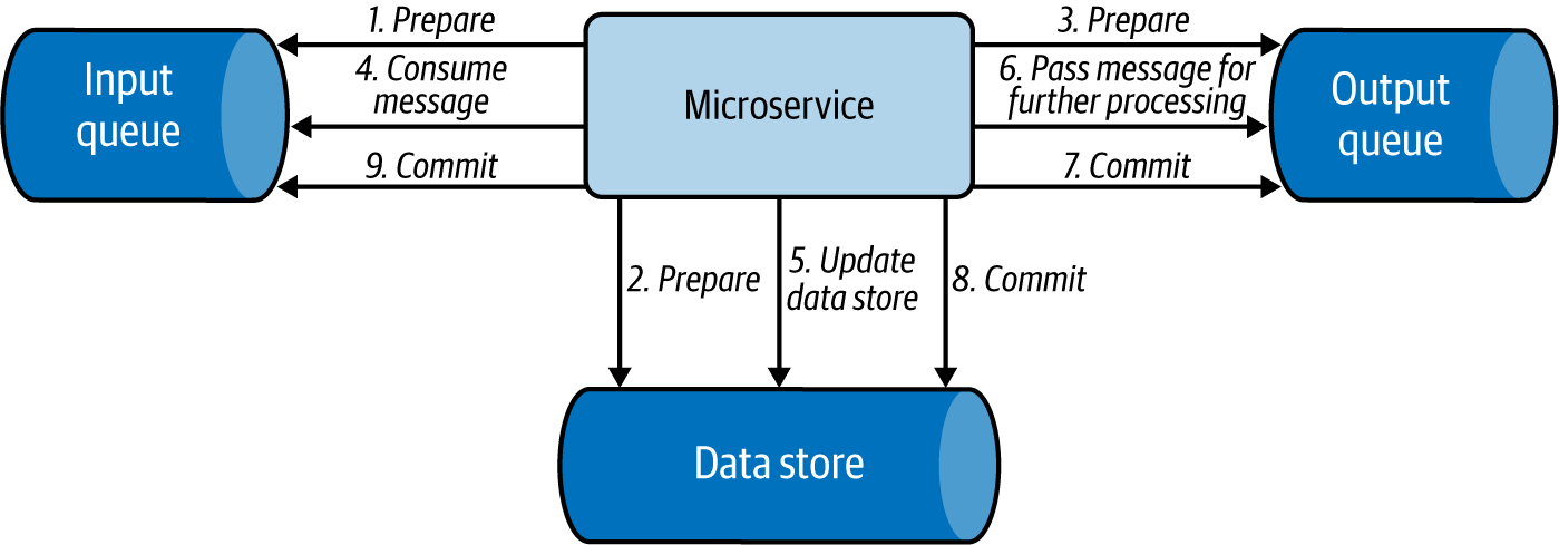
Figure 4-24. Simple message processing use case applying an XA transaction

Considerations

We do not need to use this pattern when the operation has only a single step, or when there are multiple steps but failure of some is considered acceptable.

It is important to note that the use of consensus algorithms such as XA transactions will synchronize operations and introduce latency. We recommend using this pattern only when the transaction is relatively short lived, and only if it involves few systems, as we have discussed in the order-processing example.

Whenever possible, make the operation idempotent; this will help eliminate the need for using any transactions and simplifies the system. This is because with idempotent updates, even when the same operation is performed multiple times, the results will be the same. For example, say we are always overwriting a value, such as the number of items available in the inventory. Even if we overwrite the value multiple times, it will not affect the end results. This will allow us to resend the same event multiple times to overcome system failures.

When we need to synchronize execution and have more than three systems, we recommend using the Saga pattern discussed in Chapter 3. This pattern is useful for coordinating transactions among multiple data stores, microservices, and message brokers. It enables us to execute multiple transactions in order, and to compensate previous transactions when a latter transaction fails. This can also reduce the high latency or coupling that can occur from the distributed locks used by XA transactions. But we can use Saga only when all the participating transactions can be reverted—in the event of a failure—by using a compensation transaction. This can especially become a problem when we are integrating with third-party systems and might not have a way to compensate them in the case of failure.

We recommend using XA transactions over Saga when all updates need to be done in a single data store or when all steps must be performed at the same time as an atomic operation. While Saga performs transactions in order, other systems can access data from the data stores and microservices in parallel. They can then get inconsistent results if they retrieve one part of the data from a data store that has already performed the transaction and another from a data store that has not yet processed the transaction.

Related pattern

The Transaction pattern has one related pattern, the Saga pattern. This pattern, covered in Chapter 3, reliably coordinates execution of multiple systems.

Summary of Transaction Reliability Pattern

This section outlined one commonly used pattern that provides reliability in cloud native application development. Table 4-5 summarizes when we should and should not use this pattern, as well as its benefits.

Table 4-5. Transaction reliability pattern

Pattern	When to use	When not to use	Benefits
Transaction	An operation contains multiple steps, and all the steps should be processed automatically to consider the operation valid.	The application has only a single step in the operation. The application has multiple steps, and failure of some steps is considered acceptable.	Adheres to ACID properties. Processes multiple independent transactions.

Security: Vault Key Pattern

Securing data is discussed in detail in “Security”. Here, we show how access to data stores can be controlled via the Vault Key pattern to enforce security when developing cloud native applications.

The Vault Key pattern provides direct access to data stores via a trusted token, commonly named the vault key. Some of the popular cloud data stores support this functionality.

How it works

The Vault Key pattern is based on a trusted token being presented by the client and being validated by the data store. In this pattern, the application determines who can access which part of the data.

Figure 4-25 illustrates this pattern. The client or caller service calls the application to retrieve a token to access the relevant data store. The application can be an identity provider or may contact an identity provider to validate the caller and issue a trusted vault key token for access to the relevant data store. The application can also provide a scope of operations that the caller can perform on the data store. It will also add an expiry time to the key, giving access to the service for only a defined period. The caller can then call the resource by using the given key and can perform authorized operations until the key expires.

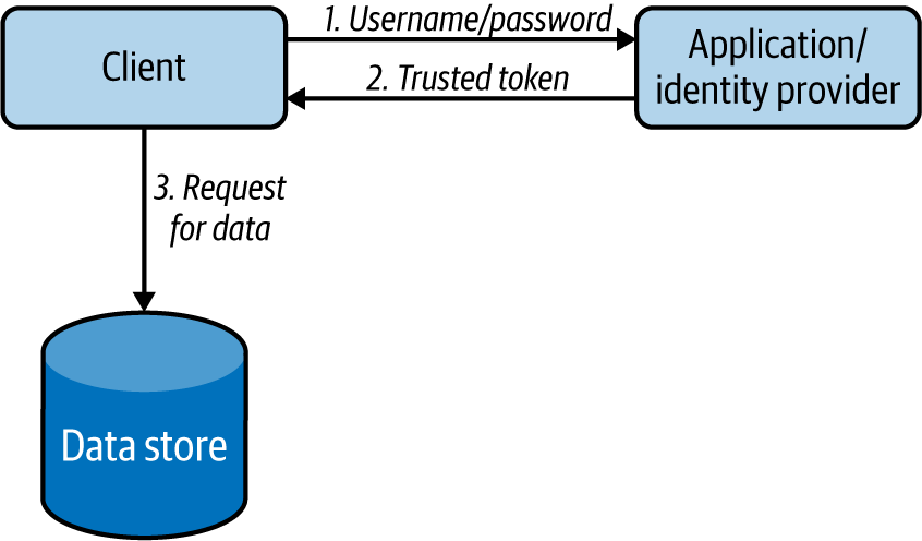
Figure 4-25. Actions performed by clients to retrieve data in the Vault Key pattern

This pattern can also support renewing the vault keys upon expiry by using a refresh token, as in API security. This facilitates smooth operation of services without getting interruptions for reauthorization.

How it’s used in practice

This pattern can be used when the data store cannot reach the identity provider to authenticate and authorize the client upon data access. In this pattern, the data store will contain the certificate of the identity provider, so it will be able to decrypt the token and validate its authenticity without calling the identity provider. Because it does not need to make remote service calls for validation, it can also perform authentication operations with minimal latency.

Considerations

Once the caller service gets access to the data store, the application that governs the service usually will lose control. This pattern provides a mechanism to withhold control over the data store and enforce security. But we can apply this pattern only when the data store supports key validation. This is important to ensure that the token is issued by the identity provider and is not expired. Some advanced data stores also support access scopes; they can identify which section of the data store, such as the table or row, can be accessed by the incoming request. When the data store can’t validate access based on keys, use alternative approaches such as fronting the stores with a data service and protecting with API security.

Sometimes the issued vault key can be compromised. In these cases, it is usually not possible to block the use of that token, as most data stores do not support this functionality. We can reduce the damage that can be caused by a compromised vault key by setting the expiry time to a moderate value.

Related pattern

The Vault Key pattern has one related pattern, Data Service (covered at the start of this chapter). Along with API security, the Data Service pattern provides an alternative approach for providing security when the Vault Key pattern is not feasible.

Summary of the Vault Key Pattern

This section outlined the commonly used Vault Key pattern, which provides security in cloud native application development. Table 4-6 summarizes when we should and should not use this pattern, and its benefits.

Table 4-6. Vault Key security pattern

Pattern	When to use	When not to use	Benefits
Vault Key	To securely access remote data with minimal latency. The store has a limited computing capability to perform service calls for authentication and authorization.	Need fine-grained data protection. Need to restrict what queries should be executed on the data store with high precision. The exposed data store cannot validate access based on keys.	Accesses data stores directly by using a trusted token, a vault key Has minimal operational costs compared to calling the central identity service for validation

Technologies for Implementing Data Management Patterns

As a software developer or architect, you have to select the most appropriate technologies for your use case. This includes selecting data stores as well. You have to select a data store based on factors such as what you are going to store, the amount of data (scalability), the expected write and read performance, system availability, and consistency. In this section, we discuss the types of data stores most commonly used for cloud native applications, and when you may use them.

Relational Database Management Systems

Most traditional databases fall under the category of relational database management systems (RDBMSs), which includes MySQL, Oracle, MSSQL, Postgres, H2, and more. These relational databases provide the ACID properties, and with their SQL can also have very complex data access patterns. However, if you have nonrelational data such as XML, JSON, or binary format, then an RDBMS may not be the best option, and you might need to select a distributed filesystem or NoSQL database to store data, as discussed previously in “Relational Databases”.

When building cloud native applications, instead of deploying the database yourself on the cloud infrastructure, we highly recommend using a managed version of RDBMSs provided by a cloud vendor, such as Amazon Relational Database Service (RDS), Google Cloud SQL, or Azure SQL. This will not only reduce the complexity of managing the databases, but also be better tuned for the environment.

To scale RDBMSs, we can deploy them as primary and replica databases, as discussed in the Materialized View pattern, or shard the data as in the Sharding pattern. In the worst case, if we still have issues with space, we can also periodically back up older, rarely used data to an archive such as NoSQL, and delete it from the store.

Apache Cassandra

Apache Cassandra is a distributed NoSQL database that began internally at Facebook and was released as an open source project in July 2008. Cassandra column store is well-known for its continuous availability (zero downtime), high performance, and linear scalability, which modern applications and microservices require. It also offers replication across data centers and geographies to guarantee availability across regions. Cassandra can handle petabytes of information and thousands of concurrent operations per second, enabling you to manage large amounts of data across hybrid cloud and multicloud environments. For cloud native application deployment, we recommend using managed Cassandra deployments such as Amazon Keyspaces and Asta on Google Cloud.

Cassandra’s write performance is very high compared to its read performance, As discussed previously in “NoSQL Databases”, it provides eventual consistency by design. However, it also lets us change its consistency levels to achieve weak or strong consistency based on the use case.

The performance of Cassandra also depends on how we store and query data. If we will be querying data based on a set of keys, we should use its row key (partition key). If we need to query data from different keys, we can create secondary indexes. Don’t overuse the secondary indexes; they can slow the data store, as each insertion has to also update the indexes. Further, Cassandra is not efficient when we want to join two column families, and we should not use it if we are to update the data more frequently.

Apache HBase

Apache HBase is a distributed, scalable, NoSQL column store that runs on top of the HDFS. HBase can host very large tables with billions of rows and millions of columns, and can also provide real-time, random read/write access to Hadoop data. It scales linearly across very large data sets and easily combines data sources with different structures and schemas.

As HBase is a column store, it supports dynamic database schema, and as it runs on top of HDFS, it can also be used in MapReduce jobs. Consequently, HBase’s complex interdependent system is more difficult to configure, secure, and maintain.

Unlike Cassandra, HBase uses “master/worker” deployment, and so can suffer a single point of failure. If your application requires high availability, choose Cassandra over HBase. However, when we depend heavily on data consistency, HBase will be more suitable because it writes data to only one place and always knows where to find it (because data replication is done “externally” by HDFS). Similar to Cassandra, HBase also does not perform well for frequent data deletes or updates.

MongoDB

MongoDB is a document store that supports storing data in JSON-like documents, as discussed in “NoSQL Databases”. Documents and collections in MongoDB are comparable to records and tables in relational databases. It uses MongoDB query language to access the stored data, perform aggregation filtering and sorting based on any document fields, and insert and delete fields without restructuring documents. MongoDB Cloud provides MongoDB as a hosted solution for cloud native application usage.

Unlike Cassandra or RDBMSs, MongoDB prefers more indexes. When not indexed, its performance can suffer, as it needs to search the entire collection. MongoDB also favors consistency over availability. It achieves availability by using a single read/write primary and multiple secondary replicas. When a primary becomes unavailable, the read/write operations will be temporarily halted for about 10 to 40 seconds while MongoDB automatically elects one of its secondary replicas as the primary.

MongoDB is heavily used for mobile applications, content management, real-time analytics, and IoT applications. MongoDB is also a good choice if you have no clear schema definition with your JSON documents, and you can tolerate some data store unavailability. However, like other NoSQL databases, it is not suitable for transactional data.

Redis

Redis is an in-memory key-value data store commonly used as a cache, as discussed in the “Caching Pattern”. It supports string keys and various kinds of values such as strings, lists, sets, sorted sets, hashes, bit arrays, and much more. This makes the application less complex, as it can now store its internal data structure directly in Redis. Redis is ideal for a cache, as it supports transactions, keys with a limited time to live, LRU eviction of keys, automatic failover, and its ability to write excess data to disk. Redis also has plenty of cloud hosting options for cloud native applications to use, including AWS, Google, Redis Labs, and IBM.

Redis supports two types of persistence options: Redis Database Backup (RDB) and Append Only File (AOF). By using both options, we can achieve good write performance and a good degree of data safety upon system failures. Redis features high availability by using a single “master” and multiple “replica"s as in the CQRS pattern, and provides scalability through sharding “master” and “replica"s as discussed in the “Data Sharding Pattern”.

However, Redis is not a NoSQL replacement for relational data stores, as it does not support many standard relational data store features, such as efficient querying, and performing complex data manipulation and aggregation operations.

Amazon DynamoDB

DynamoDB is a key-value and document database that can be used to store and retrieve data with low latency and high scalability. It can handle more than 10 trillion requests per day and more than 20 million requests per second during peaks. Data in DynamoDB is stored on solid-state disks (SSDs), automatically partitioned, and replicated across multiple availability zones. It also provides fine-grained access control and uses proven secured methods to authenticate users and prevent unauthorized data access.

DynamoDB, a service provided by AWS, cannot be installed on a local server or in clouds other than AWS. Use DynamoDB only if you are using AWS as the primary cloud infrastructure for your cloud native applications. Further, DynamoDB has limited querying capability compared to relational stores and does not support relational database features such as table joins and foreign-key concepts; instead, it advocates using non-normalized data with redundancy for performance.

Apache HDFS

The Apache Hadoop Distributed File System (HDFS) is a widely used distributed filesystem designed to run on cheap commodity hardware while providing high data resiliency by storing at least three copies of data in a distributed manner. HDFS is commonly used to store analytical data because the data stored in HDFS is immutable and is optimized to write and read data in a streaming manner. This also allows HDFS to be used as the data source for Hadoop MapReduce jobs for efficient processing of large data. Cloudera and major cloud vendors provide HDFS as a hosted service to use with cloud native applications.

HDFS stores data in multiple data nodes, and stores all its metadata in memory in a single-name node. When that node is not available, it can fail new reads and writes, causing unavailability. Also, based on the capacity of its name node’s memory, it has an upper limit on the number of files that it can store. We recommend using HDFS to store a small number of large files instead of a large number of small files. Because it is optimized to read data sequentially, it is not the best solution when we need random reads.

Amazon S3

Amazon Simple Storage Service (S3) is an object storage that is part of AWS. It can be used in a data lake, as storage for cloud native applications, as a data backup or archive, and for big data analytics. It also supports the Data Locality pattern by running analytics on data nodes using standard SQL expressions of Amazon Athena. We can use S3 Select to retrieve subsets of object data instead of the entire object. This can improve data-access performance by up to four times. Amazon S3 is highly available and provides fine-grained data access control. We recommend using it when you use AWS as your primary cloud native application platform.

Azure Cosmos DB

Azure Cosmos DB is a fully managed NoSQL data store that supports key-value, document, column, and graph database semantics. It can store and retrieve data with low latency, and provides enterprise-grade security with end-to-end encryption and access control. It also provides open source APIs for MongoDB and Cassandra, enabling clients to leverage the cloud without changing their application.

Cosmos DB, a service provided by Azure, cannot be installed on a local server or in clouds other than Azure. Use Cosmos DB only if you are using Azure as the primary cloud infrastructure for your cloud native applications. Still, Cosmos DB provides some flexibility by providing migration and synchronization of data with your on-premises Cassandra cluster. Though Cosmos DB can provide transactional support, it is limited within the logical data partition.

Google Cloud Spanner

Google Cloud Spanner is a fully managed relational data store that supports unlimited scale and strong consistency. It provides the capability to run SQL queries while providing support for transactions across all the nodes in the cluster. It also linearly scales write and read transactions and provides security through data-layer encryption and access controls.

Because Cloud Spanner is a service provided by Google, it cannot be installed on a local server or in clouds other than Google. Use Spanner only if you are using Google as the primary cloud infrastructure for your cloud native applications. Though it provides SQL support, it does not fully support the American National Standards Institute (ANSI) SQL spec and so requires changes to applications before migrating from standard relational databases to Spanner.

Summary of Technologies

This section outlined some commonly used data stores that we can use in cloud native application development. Table 4-7 summarizes when we should and should not use these data stores.

Table 4-7. Data store types

Data store type	When to use	When not to use
Relational database management system (RDBMS)	Need transactions and ACID properties. Interrelationship with data is required to be maintained. Working with small to medium amounts of data.	Data needs to be highly scalable, such as IoT data. Working with XML, JSON, and binary data format. Solution cannot tolerate some level of unavailability.
Apache Cassandra	Need high availability. Need scalability. Need a decentralized solution. Need faster writes than reads. Read access can be mostly performed by partition key.	Existing data is updated frequently. Need to access data by columns that are not part of the partition key. Require relational features, such as transactions, complex joins, and ACID properties.
Apache HBase	Need consistency. Need scalability. Need a decentralized solution. Need high read performance. Need both random and real-time access to data. Need to store petabytes of data.	Solution cannot tolerate some level of unavailability. Existing data is updated very frequently. Require relational features, such as transactions, complex joins, and ACID properties.
MongoDB	Need consistency. Need a decentralized solution. Need a document store. Need data lookup based on multiple keys. Need high write performance.	Solution cannot tolerate some level of unavailability. Require relational features, such as transactions, complex joins, and ACID properties.
Redis	Need scalability. Need an in-memory database. Need a persistent option to restore the data. As a cache, queue, and real-time storage.	As a typical database to store and query with complex operations.
Amazon DynamoDB	Need a highly scalable solution. Need a document store. Need a key-value store. Need high write performance. Fine-grained access control.	Use in platforms other than AWS. Require relational features, such as complex joins, and foreign keys.
Apache HDFS	Need a filesystem. Store large files. Store data once and reads multiple times. Perform MapReduce operation on files. Need scalability. Need data resiliency.	Store small files. Need to update files. Need to perform random data reads.
Amazon S3	Need an object store. Perform MapReduce operations on objects. Need a highly scalable solution. Read part of the object data. Fine-grained access control.	Use in platforms other than AWS. Need to run complex queries.
Azure Cosmos DB	Need a highly scalable solution. Need a document store. Need a key-value store. Need a graph store. Need a column store. Fine-grained access control. Connectivity via MongoDB and Cassandra clients	Use in platforms other than Azure. Perform transaction across data partitions.
Google Cloud Spanner	Need a highly scalable solution. Need a relational store. Need support for SQL query processing Need transaction support across all nodes in the cluster.	Use in platforms other than Google Cloud. Support for full ANSI SQL spec.

Testing

Testing is an important step for building successful cloud native applications. As we have discussed testing microservices in Chapter 2, here we will focus on testing data services and data stores.

We can use test data stores to test data-service interactions, Though data services can have complex or simple logic, they can still cause bottlenecks in production. The following are useful recommendations for overcoming these issues:

• Tests should be performed with both clean and prepopulated data stores, as the former will test for data initialization code and the latter will test for data consistency during operation.

• Test all data store types and versions that will be used in production to eliminate any surprises. We can implement test data stores as Docker instances that will help run tests in multiple environments with quick startup and proper cleanup after the test.

• Test data mapping and make sure all fields are properly mapped when calling the data store.

• Validate whether the service is performing inserts, writes, deletion, and updates on the data stores in an expected manner by checking the state of the data store via test clients that can access the database directly.

• Validate that relational constraints, triggers, and stored procedures are producing correct results.

In addition, it is important to do a load test on the data service along with the data store in a production-like environment with multiple clients. This will help identify any database lock, data consistency, or other performance-related bottlenecks present in the cloud native application. It will also show how much load the application can handle and how that will be affected when various data scaling patterns and techniques are deployed.

When it comes to testing the cloud native microservices that depend on data services, we can simply use mock service APIs to mock the data services and omit the need for deploying data stores.

Security

Protecting data and allowing only the appropriate people and systems to access relevant data is key to the successful execution of a cloud native application, and to the success of an organization in general. The security of data should be enforced both when data is at rest and when data is on the move.

We can enforce data security at rest both physically and through software. Data servers should be guarded and accessed only by authorized persons. Data stores running in the servers should also enforce security via the Vault Key pattern and API security to control data access. When storing sensitive data, we recommend encrypting it before storing it in the data store. We also recommend encrypting the filesystem in which the data is stored as an added layer of protection.

We recommend separating sensitive data from other data so that sensitive data can be governed with additional layers of protection, along with audit trails to monitor suspicious behavior. Don’t collect and store unnecessary sensitive information. When needed, mask all sensitive information such as usernames and email addresses. This can be done by replacing sensitive data with unique identifiers and storing their mapping in a protected data store. This can enable us to continuously analyze and audit user behavior while providing the capability to delete all sensitive user data by simply deleting the data mapping. This will also help enforce privacy and data regulations such as Europe’s General Data Protection Regulation (GDPR).

When it comes to data in transit, we should always transmit the data via secure data transmission channels such as HTTPS. For added security, we can encrypt the messages with asymmetric keys so that the intermediary hosts will not have access to the content.

To protect sensitive information without segmenting messages, we can encrypt only the part of the message that has sensitive information. The whole message will be delivered to each client, but only the clients with the relevant key for the sensitive data can decrypt it, while others can’t access that data.

Observability and Monitoring

Observability and monitoring enable us to gain deeper insights into the way cloud native applications are performing by looking at their metrics, logs, and distributed tracing results. As observability and monitoring of microservices are discussed in Chapter 2, here we focus mainly on data stores.

Observability and monitoring help us identify the performance of data stores and take corrective actions when they deviate because of load or changes to the application. In most applications, incoming requests interact with the data stores. Any performance or availability issues in the data store will resonate across all layers of the system, affecting the overall user experience.

Monitoring data stores is essential in order to minimize problems with performance, availability, and security. The key metrics to observe in a data store are as follows:

• Application metrics

  • Data store uptime/health: To identify whether each node in the data store is up and running.

  • Query execution time: Five types of issues can cause high query execution times:

    • Inefficient query: Use of nonoptimized queries including multiple complex joins, and tables not being indexed properly.

    • Data growth in the data store: Data stores containing more data than it can handle.

    • Concurrency: Concurrent operations on the same table/row, locking data stores and impacting their performance.

    • Lack of system resources such as CPU/memory/disk space: Data store nodes not having enough resources to efficiently serve the request.

    • Unavailability of dependent system or replica: In distributed data stores, when its replica or other dependent systems such as a lookup service is not available, it may take more time as it needs to provision a new instance or discover and route the request to another instance.

  • Query execution response: Whether the query execution is successful. If the query is failing, we may need to look at the logs for more detail (depending on the failure).

  • Audit of the query operations: Malicious queries or user operations can result in unexpected reduction in data store performance. We can use audit logs to identify and mitigate them.

• System metrics: To identify a lack of system resources for efficient processing via CPU consumption, memory consumption, availability of disk space, network utilization, and disk I/O speed.

• Data store logs

• Time taken and throughput when communicating with primary and replicas: Helps to understand networking issues and bad data store

When analyzing metrics, we can use percentiles to compare historical and current behaviors. This can identify anomalies and deviations, so we can quickly identify the root cause of the problem. For example, monitoring tools like SolarWinds and SQL Power Tools provide metrics such as query execution time and response time, and systems like Elastic Stack and Kibana analyze data store logs to illustrate their health and the reason for query failures. If we are using data stores managed by cloud vendors such as Google Cloud, AWS, or Azure, they too provide monitoring services to monitor system and data store metrics.

DevOps

We have discussed several data management patterns that can be applied in cloud native applications using both microservices and data stores. We already discussed the DevOps process for deploying and managing microservices in Chapter 2, so here we focus on deployment and management of data stores.

The steps and key considerations for deploying and managing data stores are as follows:

1. Select data store types. Select the data store type (relational, NoSQL, or filesystem) and its vendor to match our use case.

2. Configure the deployment pattern. This can be influenced by the patterns applied in the cloud native application and the type of data store we have selected. Based on this selection, high availability and scalability should be determined by answering the following questions:

   • Who are the clients?

   • How many nodes?

   • Are we going to use a data store managed by the cloud vendor or deploy our own?

   • How does the replication work?

   • How do we back up the data?

   • How does it handle disaster recovery?

   • How do we secure the data store?

   • How do we monitor the data store?

   • How much does the data store/management cost?

3. Enforce security. Data stores should be protected because they contain business-critical information. This can be enforced by applying relevant physical and software security as discussed in the preceding section. This may include enabling strict access control, data encryption, and use of audit logs.

4. Set up observability and monitoring. Like microservices, data stores should be configured with observability and monitoring tools to guarantee continuous operation. This can provide early insights on possible scaling problems, such as a requirement to rebalance data shards, or to apply a different design pattern altogether to improve scalability and performance of the application.

5. Automate continuous delivery. When it comes to data stores, automation and continuous delivery are not straightforward. Although we can easily come up with an initial data store schema, maintaining backward compatibility is difficult as the application evolves. Backward compatibility is critical; without it, we will not be able to achieve smooth application updates and rollbacks during failures. To improve productivity, we should always use proper automation tools such as scripts to automate continuous delivery. We also recommend having guardrails and using multiple deployment environments, such as development, and staging/preproduction, to reduce the impact of the changes and to validate the application before moving it to production.

By following these steps, we can safely deploy and maintain cloud native applications while allowing rapid innovation and adoption to other systems.

Summary

In this chapter, we discussed several data management patterns that can be applied to cloud native applications. We started with an overview of data architecture and then looked at various types of data such as input, configuration, and state data that can influence application behavior. We also covered forms of data, such as structured, semi-structured, and unstructured, and how we can efficiently store and manage them in various types of data stores, including relational, NoSQL, and filesystems.

We then discussed how this data can be managed and shared among cloud native applications and how to use various design patterns to achieve data composition, data scaling, performance optimization, reliability, and security. We also looked at various technologies specific to data management and how data-centric cloud native applications should be developed, tested, continuously deployed through DevOps, and observed and monitored to guarantee continuous operation. Next we will discuss patterns related to event-driven cloud native applications.