Digital Signal and Image Processing using MATLAB, Volume 1: Fundamentals, 2nd Edition

Chapter 4

Linear Filters

When building a model to describe the behavior of some of the most commonly used systems, we often rely on the superposition principle. It amounts to assuming linearity (the use of Kirchoff’s laws are an example). Usually, time invariance is also assumed. It consists of saying that, on the time scales that are used, the characteristics of these systems remain unchanged.

Linear filters are defined in the following section by these two characteristics. Because of their importance in the field of signal processing, this chapter presents their main properties, as well as a few design methods.

4.1 Definitions and properties

Definition 4.1 (Linear filter) A discrete-time linear filter¹ is a system whose output sequence results from the input sequence {x(n)} according to the expression:

(4.1)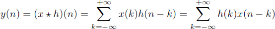

where the sequence {h(n)} that characterizes the filter is called the impulse response. The (x * h) operation is called convolution (Figure 4.1).

For example, the processing defined by y(n) = x(n) + x(n – 1) is therefore a linear filtering. The sequence {h(n)} is defined by h(0) = , h(1) = and h(n) = 0 for any value of n ≠ {0, 1}.

For commonly used classes of signals, expression ...