Scale invites complexity. Complexity breeds confusion. Confusion, in turn, increases the likelihood of error. Even more mistakes are made under pressure resulting from deadlines, the time-critical nature of the business, or high external visibility. Timely response to production issues becomes more difficult at scale.
Some amount of complexity is unavoidable, so striving for simplicity, while a good thing in itself, is not the same as achieving it. Likewise, working under pressure is not something that will go away anytime soon. When is the right time to expand the team? Then again, the more people on the team, the harder it is to maintain consistency.
Increasing a system’s manageability is a sure way to counter these factors. Rich instrumentation is a necessary yet not sufficient condition. If your system is expanding, this chapter might help you in planning an alerting configuration that scales along with it. If you have already reached the critical mass and monitoring is starting to become increasingly more complicated, this chapter will help you get back on track. It describes best practices for developing managed alerting configurations.
Large-scale information systems consist of numerous groups of interconnected computers. Their numbers start in the region of hundreds and go beyond tens of thousands. To improve resilience, availability, and access times, the systems may be distributed in diverse locations across the world. The computers communicate over a best-effort network, reliability of which cannot be taken for granted. The more complex hardware pieces the system consists of, the higher the possibility of failure in one of the individual parts. At a large scale, failure is not unusual.
Operating large systems comes at a cost. Their operation typically provides an important service and generates significant revenue streams. Any moment of downtime brings down the service and translates to losses. This makes failures in big systems highly visible, not only within the organization that runs them, but also in the media if the system provides a popular public service.
It is for that reason that organizations operating at large scale put great emphasis on preventative measures. They can include investigations into anomalies and atypical usage patterns aimed at ruling out any possibility of problem escalation. In low-visibility organizations, on the other hand, it is somewhat acceptable to respond to alerting events in a reactive rather than proactive way. It is also permissible in small settings to close up shop for an upgrade and ask users to come back later. The same is not an option in big systems. They require staggered, continuous maintenance, carefully carried out in phases.
Information systems process and store data to extract specific meanings. Raw data enter the system with various, sometimes unpredictable frequencies and the outcome of processing takes different forms. Processed data may be volatile and lose validity within minutes, as in the case of short-lived stock market price projections or relevance suggestions on a social networking site. Other processed data may be long-lived and relatively bulky to store, such as video clips on a broadcasting website. A system’s architecture is shaped by existence and values of many such values, including data volatility and the cost of retention.
The designer makes a series of trade-offs, giving up efficient utilization of one resource in order to accommodate better utilization of a more essential resource. As a result, specific purpose systems are well suited for solving one kind of a problem but not the other—and some of their components will always be more prone to failure than others. An overall calculation of a system’s durability should put the most weight on the durability of its weakest link.
In busy production environments with data processing rates of terabytes per second, the Law of Large Numbers applies. This makes their monitoring a great learning opportunity. Data generated at such magnitude of scale approximates mathematical models very closely and assumptions can be made with higher confidence. On the other hand, even small changes, assumed to cause disruption at seemingly negligible levels, might affect thousands of users. Even small mistakes can become highly visible. Finding out about faults from your users is never a good place to be. This is yet another reason for special care in carrying out daily operations and the need for fine-grained monitoring.
Finally, delays tell the story. Increased network latencies and system response times indicate overall performance degradation. Time delays can be seen as the most universal currency of performance. Small increases in response times might be an indication of increased load, but when delays rise to exceptionally high levels, they become a serious problem. Users tend to respond immediately by demonstrating their lack of patience. Internet giants are extremely sensitive to latency because it directly affects their bottom line.
Less pronounced shifts in delay time patterns might not always have a direct impact, but they do point to potentially worrisome changes downstream in the solution stack. Big systems supply enough inputs to reliably detect subtle changes. Detecting and dealing with them remains a focus of operations at scale.
Considering these aspects of large systems, a set of assumptions about the operation of large-scale systems can be drawn.
Data enters and leaves with varying intensity and frequency, both of which are subject to a high degree of unpredictability.
The scale of operation necessitates continuous maintenance.
Increases in response time and latency adds costs to the organization.
The longer the component interdependency chain is, the higher the likelihood of hitting a bottleneck.
Failures are inevitable; they are the norm. The aim is to minimize their effects.
Data flow in a system is often compared to fluid conveyance in a set of pipes. The data is encapsulated in the form of messages and continuously passes through the system. Large information systems are composed of subsystems made up of components, which in turn are subdivided. The requests are routed between components according to some application logic. Components in each subsystem take different functional shapes, including but not limited to the following:
- Service interface
The way to take in and serve data, most frequently in the form of requests and responses. Interfaces can be read-write to allow submission of data, or read-only, meant exclusively for data consumption. Present day services are commonly built on top of a well defined HTTP interface.
- Data processor
Software that extracts selected aspects of information from the data and presents it in an alternative, usually more compact form. Processors may be real-time or offline, for example, a search result rank calculator or a map-reduce cluster.
- Data pipeline
A serial chain of specialized data processors and transformers, taking a data stream at the ingress and returning it processed at the egress. Pipelines are built with continuity of data processing in mind and their end-to-end latency of processing is optimized to be as short as possible.
- Datastore
A repository of data objects designed for specific access and persistence patterns. Examples include databases, network filesystems, shared storage systems, and cache fleets.
In order to meet the load and provide basic redundancy, the components are deployed to groups of hosts, or server fleets. Placing any of the components on a single server creates a Single Point of Failure (SPoF) because a failure of a single machine can be responsible for an entire system stopping its functionality and postponing operation. SPoFs must, therefore, be avoided.
The components of an application may be loosely or tightly coupled; the service interface and data processor may operate as separate fleets of hosts, but it is not uncommon to see them run out of the same server. Decoupling helps isolate failures, but introduces additional cost and overhead in data transmission. Each component is a computational platform consisting of a hardware and software stack. If components are coupled, it means that they share a portion of the platform at least up to the operating system layer. This has important implications for fault finding: an intensive utilization of resources by one component might slow down another.
A system in distributed operation is a bunch of computers collaborating on the network. While the computers are not necessarily plugged into each other in any particular order, a system’s logical architecture does depend on how the data is processed, the frequencies at which it enters and leaves the system, and in what form. Some systems crunch big data sets, others are expected to produce meaningful result in real-time, and yet others are developed with persistence in mind to provide distributed storage for high-availability of data retrieval. Regardless of the purpose, a system’s composition should be clearly defined in terms of its fundamental components, their coexistence, and architectural layout. Such a layout map serves as a base for establishing what areas should be covered by monitoring, and in case of failures it may serve as a reference guide for operators who are not familiar with the system intimately.
Effective alerting configurations are rare. Most of them come with time, often built through trial and error. Interestingly though, they all share the same three characteristics: the thresholds are cleanly ordered, data-driven, and reevaluated when baselines shift. These rules apply to systems of any size, but their value becomes truly apparent in large and complex settings, where the system evolves, maintenance is laborious, and alarm thresholds are a moving target.
- Order
Highly manageable large-scale systems are organized hierarchically and benefit extensively from the use of namespaces. Such a structured organization of alarms empowers the operators to work with alerts with more effectively.
Consistent namespacing allows for reliable audits and facilitates housekeeping. Alarms may be reliably classified as stale or obsolete if they don’t reflect the current configuration or hierarchy of the system. Such alarms may subsequently get cleaned up to reduce their maintenance cost and prevent confusion among engineers. Additionally, order simplifies the task of setting up aggregation and suppression, and is a major factor behind alerting’s effective manageability.
- Data-Driven Organization
Timeseries data stores valuable information about the long-term process of change. This information should be used to drive alarm thresholds, as explained in Data-driven thresholds.
Threshold values, calculated from historical observations, anchor alarm behavior at real data. Some metrics produce continuous streams of data. These may oscillate around an almost constant value or be subject to seasonal cycles. Other metrics yield occasional spikes, not all of which indicate real issues. The baseline, the magnitude of failure, and the existence of anomalies should all be taken into account. A sound and reproducible calculation model leads to stronger detectability and reduction in human effort. The applicability of each calculation model is tied to the underlying data patterns, but they’ll nearly always do a better job than a human.
- Reevaluation
Many things will change over time, starting with hardware and infrastructure, through code efficiency, ending with traffic patterns. Although not all changes come at once, they will arrive eventually. In reality some changes are more progressive than others, and some configurations require a rich granular set of alarms while others do not. For that reason, different groups of alarms require reevaluation at different time intervals. When monitor thresholds are refreshed regularly to adjust to changes in usage patterns, alerting becomes significantly more sensitive and specific.
Large, manageable systems are organized in hierarchies, grouped by components and their relevant logical entities, according to the number of abstract dimensions that they operate in. The resulting software stack is then replicated to multiple locations around the world. In this context, a dimension is a way of presenting measurements that reflects the system’s architecture and location. Full monitoring coverage should reflect as many dimensions as there are in the system.
Consider a simplistic model of a three-tier system expressed in terms of its dimensions, depicted in Figure 4-1.
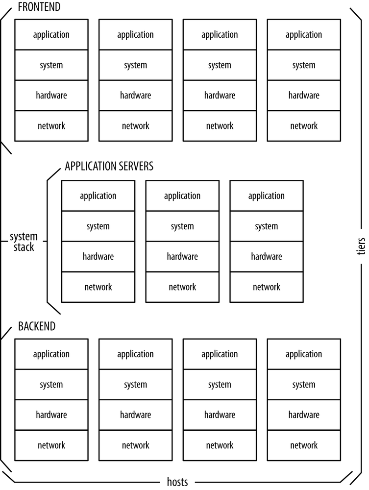
Dimension 1: covering each of the three tiers—the front end, the application layer, and the back end
Dimension 2: vertically spanning the layers of hardware and solution stack
Dimension 3: all server entities
Effective monitoring should cover all components of a system at its many levels of granularity. The operator must be able to get an immediate insight into parts of the system where faults are suspected, zoom in or out into arbitrary levels of data granularity, and overlay cross-layer metrics freely to highlight correlative relationships. You need to realize the kinds of structures shown in Figure 4-1 in order to make reliable assumptions.
Big systems with comprehensive monitoring collate millions of inputs into hundreds of thousands of data points per minute. Most of them will never get looked at. The penetration rate of metric data in large enterprises is estimated to be around 1%—and that’s okay, because most of the monitoring data is collected just in case, for real-time inspection during an event response. In reality, only a small fraction of timeseries is constantly monitored by alarms and through dashboards and even fewer of them will be used for long-term analysis of seasonality trends.
When a need arises, the operator must know how to find her way through the remaining 99% of metrics in search of the defects. Data must be reported systematically. The question is how to report and store metrics so they can be retrieved with minimum effort and, in the process, discovered intuitively.
The way to do this is by storing the data so as to reflect a system’s dimensions. In other words, every data input consists of a numeric value and a set of properties describing its origin and the circumstances under which the input was collected. All these properties can be seen as dimensions and their values can be interpreted as data addresses in an abstract multidimensional space. Through referencing data by their properties and origin, specific subsets of recorded inputs can be carved out from a metric and presented in the form of a timeseries.
Let me explain this idea by expanding a little on the example from Figure 4-1. Suppose we have three groups of hosts representing the front end, middleware, and the back end. The hosts report their average CPU utilization at one minute intervals. Front-end machines take HTTP requests from the users and dispatch the logic to middleware, which in turn engages the back end to do some heavy lifting. When the process is finished, the middle layer fetches the result from the back end and passes it on to the front end to be served back to a user.
All three groups contain a different number of hosts, according to the frequency and intensity with which they carry out their tasks. Each host sends CPU measurements marked with the hostname of origin and the group the host belongs to.
A distributed system is typically composed of hundreds if not thousands of logical components performing some type of work. Present-day systems scale with demand, so some parts might be more volatile than others. In addition, enterprise-level alerting systems are extremely feature-rich, so learning to operate them effectively takes a bit of experience and some attention. The former comes with time (which in itself is a scarce resource), and the latter is split among many other aspects of work. In addition, rich features often give the operators enough rope to hang themselves. This poses an important question: how to maintain desired coverage without burdening operators with the nontrivial, yet mundane and unreliable process of manual updates? Let me break down the problem of alerting at scale into smaller components expressed in terms of monitoring.
- Coverage
Relying on human operators for setting up complex alerting configurations through makeshift scripts is inherently unsound. The system may be composed of moving parts. Unless the operator remembers to amend the configuration after every change, the coverage will deteriorate. This reduces the reliability of detecting alarms.
- Detectability
Coming up with threshold values is not a trivial task. The process is often counterintuitive, and it’s simply not feasible to carry out an in-depth analysis for a threshold calculation on every monitored timeseries. A data-driven approach to setting up alarms significantly improves precision.
- Consistency
The value of consistency seems a little abstract, but it is very real. A consistent convention for the structure of alarms drives simplicity and allows for predictability. It can serve as a common interface to read-only information about the current system’s state. Chapter 5 explains how to realize this potential through system automation.
- Maintenance
The creation of thousands of alarms and monitors is a labor-intensive task. When a system is cloned to another availability zone, or some parts of it are copied or expanded, a significant amount of work has to be put in reproducing its alerting configuration. The same goes for tearing down alarms: cruft (irrelevant or outdated code) builds up over time. Cruft doesn’t always incur direct costs, but it is often a source of unnecessary confusion. Any attempt to do manual clean-ups introduces the likelihood of accidental damage to the functioning configuration.
The answer to complexity lies in the automation of the process in a way that detects changes in system layout and acts on them before a human operator would. Automation makes alarms systematic and greatly simplifies the preservation of reliable coverage, detectability, and consistency. Additionally, it takes away human effort. Using a managed solution saves lots of operations time, but its most important benefit is a systematic approach to making monitoring better. The change is perceivable by everyone on the team and can be reliably measured with the methods described in Chapter 7.
When the system reaches a certain size, work invested in monitoring may become excessively laborious due to the complexity of the system combined with high rates of change. To solve the problem, the following issues must be addressed directly.
The alarm setup should reflect the logical topography of the system. Giving alarms namespace-like names brings order and allows you to maintain a hierarchical view. Namespacing provides a convenient abstract container and helps you divide and conquer huge amounts of independent monitors and alarms by functional classification. It’s a much better idea to give your alarms systematic rather than descriptive names, such as “All throttled requests for the EU website.”
Let me explain this with the familiar three-tier system example. Suppose the system provides some data crunching web service and is located in Europe. The three tiers—front end, middleware, and back end—each run on a separate fleet of hosts. Let me call them frontend, app, and db. Now, assume you want to measure CPU utilization and response latencies in each of the tiers. You could build the structure of alarms and give them names according to the following convention:
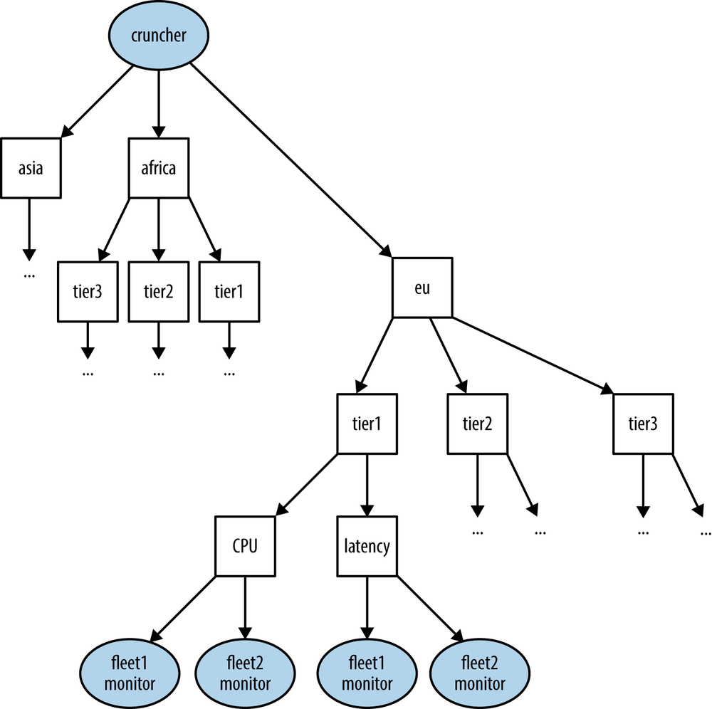
<service name>.<location>.<tier>.<alarm type>.<alarm>[.<monitor>]Figure 4-2 illustrates the breakdown of alarms. For instance, cruncher.eu.frontend.cpu-util.critical would be the name of an alarm for critical CPU utilization levels on the frontend tier in EU’s instance of “cruncher.” If you wish to expand the system to serve another geographical region, the overall alarm structure and naming convention would remain the same. Only the location identifier in the namespace would change.
This approach is very powerful. Consistently named alarms provide efficient reporting, ease maintenance, and open the door for using monitors as inputs in automation. Let me point out just a few examples:
Low-level alarms or their aggregates can be used as suppression rules for higher level alarms.
Transparency into alarms’ coverage increases because the alarms may be listed by prefix or regular expression.
The need to remember alarms by name is replaced by understanding their structure.
If monitored timeseries are subject to changes in patterns, be it sudden or progressive, their thresholds should be anchored at baselines to reflect the most recent system state. This approach makes detection significantly more accurate.
Imagine that our example system accepts three types of requests for data crunching: small-frequent, medium-regular, and big-infrequent. Let’s assume that the frequency of submission corresponds to the strain of the front end and that the size of requests dictates the load on the back end. The bigger the requests, the less frequently they come in. Suppose you monitor front-end traffic to predict back-end load. In order to do it accurately, you need different thresholds for each type of request, since a few extra big requests have the same effect on load as a huge uptake of small requests.
When the system deals with hundreds of logical entities, each with different load and usage patterns, it’s impossible to select a silver-bullet threshold. In such cases, each timeseries is treated as a special case and should get a custom threshold calculated for it.
Where possible, the method of calculation ought to reflect the underlying pattern. For instance, where you want to catch small and relatively infrequent deflections from a steady norm, a threshold based on average of data points and their standard deviation might be most appropriate. For other cases, long streaks of low data points may be discovered by watching for continued occurrences of data points below last week’s median or p40 value. A practical, universal method for many use cases was discussed in more depth in Data-driven thresholds.
Setting up data-driven thresholds requires their periodic readjustment. Depending on the frequency with which the system gets upgraded, the varying quality of infrastructure, and the system’s usage intensity, the metrics will demonstrate changes in patterns at different intervals. The idea is to keep the thresholds coherent with values of the underlying timeseries baseline.
Periodic recalibration also responds to the second type of change, one in the system’s internal structure. With time, some parts of the system might go away, while other branches might expand. In the former case, refreshing the alarms is a great opportunity to get rid of cruft, while the latter allows you to extend alerting coverage to the new parts of system.
This section attempts to provide a brief specification for creating a small framework that will help you manage thousands of alarms effectively. It combines the previous chapters into a concrete, practical solution, a basic implementation of which should not exceed 400 lines of code in your favorite scripting language.
Think of the solution as a black-box framework composed of two parts: configuration modules and an engine for refreshing the alarms that they describe. The framework is meant to glue together and extend the functionality of your existing monitoring and alerting platform to make maintenance of thousands of alarms a manageable and effortless process.
It breaks the whole configuration down in three hierarchically ordered concepts:
Configuration modules with specifications of related alarms, organized in period groupings
Alarm specifications describing alarms as groups of monitors and time evaluations aggregated accordingly
Monitors pointed at specific timeseries with thresholds calculated according to alarm specification
In its simplest form, the solution can be implemented as a periodically running cron job executing a triple nested “for” loop. The loop iterates over the creation of monitors for each alarm, all alarms for each configuration module, and all modules in a refreshment interval grouping.
The result of the operation is a consistent alarms setup. All alarms and monitors are given namespace-like names, leaving the setup in an ordered, hierarchical structure.
The remainder of this section assumes the ability to programmatically interface with the monitoring and alerting platform, in particular:
To read timeseries data
To create and delete alarms and monitors
To list existing alarms and monitors
The task of the engine is to periodically refresh alarms according to their specification. It implements reusable procedures for threshold calculation, alarm setup, and alarm tear-down to provide the following core functionality:
Interpretation of configuration modules
Plugging into the monitoring platform to manipulate alarms and monitors according to their specification. This includes their creation, modification, and deletion.
Calculating thresholds from historical timeseries data with at least one method. An idea for a robust method and simple implementation was presented in Chapter 3.
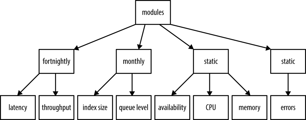
Alarm refresh intervals are central to the concept of managed alerting. Alarm groups are classified by the frequency with which their monitor configuration is to be reevaluated. I recommend four practical refresh intervals:
- Weekly
This is useful for data inputs that change frequently and are critical to the system operation. You should typically set up a relatively small number of alarms against their monitors. A weekly refresh interval is particularly suitable for systems that run on aggressive release schedules, such as continuous integration.
- Fortnightly
Similarly to weekly metrics, monitors set up around metrics susceptible to progressive changes in usage patterns should be updated every two weeks, in particular if the changes are caused by uncontrollable external factors, such as traffic levels. If a weekly module defines thousands of alarms to readjust, it makes sense to also place it in the fortnightly grouping.
- Monthly
This interval is suitable for metrics reflecting the sustained growth of relatively abundant resources, such as the levels of storage consumed by the customer.
- Static
A certain group of monitors does not need periodic adjustments because static thresholds reliably describe them. These alarms are still subject to automatic setup and tear-down, but only once—at software roll-out time. Monitors with static thresholds can be set up for watching utilization limits, loss of availability, or discontinuation of flow. Static thresholds discusses these examples in more detail.
Figure 4-3 shows how some resources might be classified.
The engine gets kicked off periodically from cron. In practice, refresh intervals are groupings of configuration modules. When the engine gets started, it is instructed to process modules belonging to one particular group. All modules from that group are loaded and interpreted, and their configuration is subsequently refreshed. See Figure 4-4 for the process.
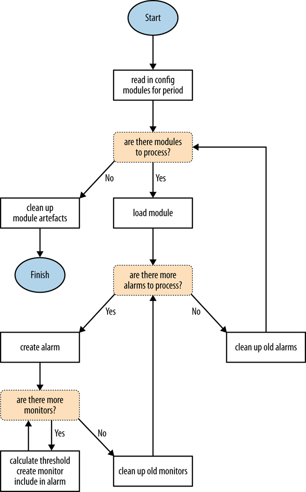
The nested loop should carry out three tasks: naming alarms, calculating monitor thresholds, and cleaning up artifacts.
The engine should construct the namespace name for alarms and monitors as follows:
<prefix>.<module>.<alarm>[.<monitor>]where the elements of the name are as follows:
prefixAn identifier specific to the system. The prefix can be a simple word (“website,” “cruncher”) or a combination of words describing the system and its properties (“website.eu”).
moduleThe name of the module containing alarm specifications, (“cpu-util,” “network”).
alarmThe name of an alarm aggregate described by each alarm specification.
monitorThe name of member monitor in the alarm aggregate.
For each defined alarm aggregate and its corresponding monitors, the engine should be able to:
Identify the timeseries for each monitor, extract its recent data points, and calculate a threshold according to specification (see Chapter 3 for a universal threshold calculation method).
Create the monitor and aggregate it in the parent alarm through one of the aggregation methods (Any, All, or By Count).
Optionally, outfit the alarm with alerting and ticketing action.
Having read the configuration of the module, the engine should be able to compare the desired configuration state with the current one, created by the previous iterations.
If more monitors are observed after an iteration of each run than are defined in the specification, the excessive monitors can be identified by name and removed. If an alarm specification got removed from the module, this fact should also be detected and the corresponding alarm with all its monitors should be cleaned up.
Modules are pieces of configuration used in the loop to set up alarms. They list and describe alarm specifications, including the alarm name, its monitors, the type of aggregation, and the alerting configuration. The information extracted from the modules describes the alarms to be created in detail. Such alarm specifications include the following:
Alarm name.
Monitor names and handles for timeseries on which one or more monitors will be based.
Alarm aggregation type (“Any,” “All,” or “By Count”).
Threshold calculation tactic. The threshold may be static or adjustable based on recent data point patterns.
Alerting information: notification action and ticket definition.
Very often a single alarm may be supported by a number of
monitors. Each monitor relates to the same metric but watches its
own dimension. This is why the definition of a timeseries to be
monitored should support some basic templating functionality. The
following example substitutes the '$(MONITOR)' placeholder in the timeseries
template with the respective monitor name. This way, having defined
the metric and timeseries just once, you can create a number of
related monitors, differing only by the one dimension in the
$(MONITOR) placeholder.
Consider the following content returned from a configuration module called “workload”:
{'utilization':{'timeseries':{'metric':'cpu-util','dimensions':{'tier':'backend',},'summary stat':'avg',},'monitors':['critical'],'aggregation':'ALL',# Not really needed for a single monitor.'threshold':{'trigger':'above','datapoints':4,# Alarm after 4 data points'static':0.80,# Trigger when the level raises above 80%},'ticket':{'title':'Critical levels of CPU utilization.','description':'Backend fleet CPU util exceeded 80%','impact':2,# Real threat of possible performance degradation.},},'traffic':{'timeseries':{'metric':'requests','dimensions':{'request_type':'$(MONITOR)',},'summary stat':'n',},'monitors':['small-frequent','medium-regular','big-infrequent'],'aggregation':'ANY',# Trigger if any of the monitors go into alert'threshold':{'trigger':'above','datapoints':5,# Alarm after 5 data points of unusually'percentile':98,# high traffic levels. Do not let the threshold'lower':50,# fall below 50 data requests per data point and'upper':1000# don't let it raise beyond 1000 requests.},'ticket':{'title':'Unusually high traffic levels for last 5 data points.','description':'One or more request types come at increased rates.','impact':3,# Real threat of possible performance degradation.},},}
The configuration describes two alarm specifications.
The first alarm is called “utilization” and contains a single monitor. The monitor watches fleet-wide CPU utilization of the back end and goes into alert state if the threshold of 80% is exceeded for 4 data points. When that happens, the alarm is instructed to file a ticket of relatively high priority.
The second alarm is called “traffic” and includes three monitors observing the number of requests per data point. Because the three types of requests have different usage patterns, threshold values for their monitors are allocated dynamically, based on the 98th percentile in the distribution of historical data points. It was established that a threshold value of below 50 should never be considered a threat, and at the same time, the value should never drift beyond 1000 for any of the monitors. If any of the monitors goes into alert state, a normal priority ticket is filed.
The process executing the loop glues together elements of the namespace to come up with a full name for every monitor and alarm that it creates. It puts together the system name (prefix) with names for module, alarm, and monitor, delimiting them with dots. That way, the CPU alarm handle becomes “cruncher.workload.utilization.critical” and the traffic monitor of the small and frequent type of requests is alarmed on via “cruncher.workload.traffic.small-frequent.”
The value and applicability of suppressions was explained in Suppression. Manually suppressing large alerting configurations for hundreds of alarms is a mundane and inconvenient task. Seeing alarms as Boolean functions, it is really simple to implement suppression functionality by appending to the aggregate the AND NOT condition pointed at a suppressing condition. That way, through changing a state of a single alarm, alerting for an entire component could be put on hold and an alert storm could be avoided.
Consider the following configuration for the data pipeline discussed in Case Study: A Data Pipeline.
Example 4-1. Simple alerting configuration returned from the “pipeline” module
{
    'throughput': {
        'timeseries': {
            'metric': 'processed_items',
            'dimensions': {
                'component': '$(MONITOR)',
            },
            'summary stat': 'sum',
        },
        'monitors': ['loader', 'processor', 'collector'],
        'aggregation': 'ANY',
        'threshold': {
            'trigger': 'below',
            'datapoints': 1, # Alarm as soon as the pipeline stops
            'static': 1, # Trigger when no items are processed
        },
        'ticket': {
            'title': 'Data pipeline has stopped.',
            'description': 'Unexpected pipeline stoppage.',
            'impact': 2,
        },
        'suppression': 'cruncher.suppressions.pipeline.maintenance'
    }
}
The resulting configuration is a single alarm, cruncher.pipeline.throughput, consisting of three monitors aggregated in ANY mode. The alarm goes into alert if any single monitor triggers. The threshold condition is set as static and goes off when the number of processed items in the data point is less than one, i.e., when it is equal to zero. This is desired except when scheduled maintenance is to be carried out, during time which the pipeline stops for a short time under full control and supervision.
The final ‘suppression’
keyword could be interpreted by the engine as attenuating
circumstances in which the alarm should not be set off after all.
The logical Boolean resulting from the configuration could be
expressed as follows:
See Figure 3-3 for a visual representation. In other words, trigger if any of the monitors is set off unless a suppressing alarm exists and is in alert state.
Tip
To make the suppression process fully hands-off, you should extend the pipeline shutdown procedure programmatically to put the cruncher.suppressions.pipeline.maintenance alarm in alert state for the expected duration of the outage, e.g. 1 hour. This way, the operator’s only worry is to carry out maintenance and not to deal with instrumentation, which further shortens the expected downtime.
Okay, let’s kick the requirements up a notch. Let’s say you want to create a more sophisticated configuration, with a separate alert for each component as illustrated in Figure 3-4. Additionally, you want the monitors to be more intelligent so they can also detect exceptionally low levels of throughput, as opposed to just an absolute discontinuation of flow. Suppose you don’t want the pipeline to go any slower than the slowest 5% of performance for a duration of three data points. Still, you want to use common sense limits for both thresholds: the lower at 1 and the upper at 100. This means that if the lowest 5% of historical performance turns out to be 0 items per data point, disregard it and use 1 instead. If, on the other hand, the slowest 5% of data points point to a performance of 100 items per data point interval, stick to the maximum threshold value of 100. Example 4-2 describes this configuration, using the analogy of Example 4-1.
Example 4-2. Granular alarms with calculation of throughput threshold for each component
{'loader': {'monitors': ['throughput'],
            'suppression': 'cruncher.suppressions.pipeline.maintenance',
            'threshold': {'datapoints': 3,
                          'lower': 1,
                          'percentile': 5,
                          'trigger': 'below',
                          'upper': '100'},
            'ticket': {'description': 'loader is unexpectedly slow.',
                       'destination': 'teamloader',
                       'impact': 2,
                       'title': 'loader has stopped.'},
            'timeseries': {'dimensions': {'component': 'loader'},
                            'metric': 'processed_items',
                            'summary stat': 'sum'}},
 'processor': {'monitors': ['throughput'],
               'suppression': 'cruncher.suppressions.pipeline.maintenance ' + \
                              'OR cruncher.pipeline.loader.throughput',
               'threshold': {'datapoints': 3,
                             'lower': 1,
                             'percentile': 5,
                             'trigger': 'below',
                             'upper': '100'},
               'ticket': {'description': 'processor is unexpectedly slow.',
                          'destination': 'teamprocessor',
                          'impact': 2,
                          'title': 'processor has stopped.'},
               'timeseries': {'dimensions': {'component': 'processor'},
                               'metric': 'processed_items',
                               'summary stat': 'sum'}},
 'collector': {'monitors': ['throughput'],
               'suppression': 'cruncher.suppressions.pipeline.maintenance ' + \
                              'OR cruncher.pipeline.processor.throughput',
               'threshold': {'datapoints': 3,
                             'lower': 1,
                             'percentile': 5,
                             'trigger': 'below',
                             'upper': '100'},
               'ticket': {'description': 'collector is unexpectedly slow.',
                          'destination': 'teamcollector',
                          'impact': 2,
                          'title': 'collector has stopped.'},
               'timeseries': {'dimensions': {'component': 'collector'},
                               'metric': 'processed_items',
                               'summary stat': 'sum'}}}
All is well, but at three components the configuration starts
getting lengthy. If the pipeline was extended by another two
components, maintaining this configuration would become a real
maintenance burden. This is precisely why static configuration files
should be replaced by executable configuration modules, which are
easier to maintain and can figure out system settings on the fly.
See Example 4-3. The imported
get_components function is assumed to be a part of a
system’s programmatic interface that can read the list of components
at the time when configuration is compiled.
Example 4-3. Module generating alerting configuration
from system.pipeline import get_components
# get_components() returns a tuple with component names.
# The following code is assumed:
# def get_components():
#     return ('loader', 'processor', 'collector')

alarms = {}
components = get_components()

for i in range(len(components)):
    alarms[components[i]] = {'monitors': ['throughput'],
        'suppression': 'cruncher.suppressions.pipeline.maintenance',
        'threshold': {'datapoints': 3,
                      'lower': 1,
                      'percentile': 5,
                      'trigger': 'below',
                      'upper': '100'},
        'ticket': {'description': components[i] + ' is unexpectedly slow.',
                   'destination': 'team ' + components[i],
                   'impact': 2,
                   'title': components[i] + ' has stopped.'},
        'timeseries': {'dimensions': {'component': components[i]},
                        'metric': 'processed_items',
                        'summary stat': 'sum'}}
    if i:
        alarms[components[i]]['suppression'] += \
            ' OR cruncher.pipeline.%s.throughput' % components[i-1]
print alarms
That’s much shorter! Additionally, when the pipeline is extended by the fourth component, the generated configuration will take this fact into account and automatically create an alerting configuration for it, too. This way, there is no need for dispatching update tasks to an operator, no one has to review it for correctness, and there is no obligation to schedule tasks to push out production changes—the alerting configuration should get regenerated the next time the loop runs to refresh alarms.
On top of core functionality, the engine may optionally also implement the following:
Distributed execution. The periodic update of thousands of monitors supporting hundreds of alarms may necessitate staggered update of alarms from multiple hosts for added reliability and to distribute load on internal monitoring tools.
The ability to calculate a threshold value for one timeseries, based on data points from a related timeseries. Sometimes the threshold value for one timeseries monitor might be calculated most reliably from data points of a related timeseries. Thus, if you want to alarm when errors exceed 1% of overall traffic, you’re setting up the error series’ threshold based on a calculation of healthy traffic.
Suggesting the severities and threshold levels for tickets based on human feedback from the ticketing system (supervised learning).
and much more!
The result of applying the proposed solution is a hierarchically ordered structure of highly effective alarms with increased sensitivity and specificity. Let me provide some anecdotal evidence.
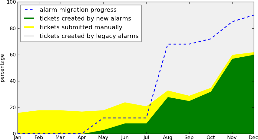
One of the operations teams I worked for introduced this form of managed alerting by implementing a simple engine and slowly migrating a portion of alarms. Figure 4-5 is a rough illustration of the progress as it was taking place during the switch-over. The yellow streak signifies human-created tickets. The green area at the bottom right is the relative amount of tickets created with the managed solution and the gray area at the top represents automated tickets created by legacy settings. Finally, the blue-dotted line reveals in percentage terms the number of alarms migrated to the managed solution. In the end, 85% of migrated alarms produce only 54% of overall tickets. Even with human created tickets taken away, we achieved a noise reduction of more than 23%. Also, notice how the streak of manually created tickets keeps decreasing during the transition—a clear indicative of improved recall.
Get Effective Monitoring and Alerting now with the O’Reilly learning platform.
O’Reilly members experience books, live events, courses curated by job role, and more from O’Reilly and nearly 200 top publishers.

