Most people don’t need much convincing to use Excel, Microsoft’s premier spreadsheet software. Its overwhelming popularity, especially in the business world, makes it the obvious choice for millions of number crunchers. But despite its wide use, few people know where to find Excel’s most impressive features or why they’d want to use them in the first place. Excel 2010: The Missing Manual fills that void, explaining everything from basic Excel concepts to the fancy tricks of the trade.
This book not only teaches you how Excel works, but also shows you how to use Excel’s tools to answer real-world questions like “How many workdays are there between today and my vacation?”, “How much money do I need in the bank right now to retire a millionaire?”, and “Statistically speaking, who’s smarter—Democrats or Republicans?” Best of all, you’ll steer clear of obscure options that aren’t worth the trouble to learn, while homing in on the hidden gems that will win you the undying adoration of your coworkers, your family, and your friends—or at least your accountant.
Note
This book is written with Microsoft’s latest and greatest release in mind: Excel 2010. This book isn’t the best choice if you’re using an earlier version of Excel, because Microsoft is continually changing Excel’s user interface (the “look and feel” of the program). To get the right instructions, look for a previous edition of this book, such as Excel 2007: The Missing Manual or Excel 2003: The Missing Manual.
Excel and Word are the two powerhouses of the Microsoft Office family. While Word lets you create and edit documents, Excel specializes in letting you create, edit, and analyze data that’s organized into lists or tables. This grid-like arrangement of information is called a spreadsheet. Figure 1 shows an example.
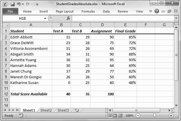
Figure 1. This spreadsheet lists nine students, each of whom has two test scores and an assignment grade. Using Excel formulas, it’s easy to calculate the final grade for each student. And with a little more effort, you can calculate averages and medians, and determine each student’s percentile. Chapter 8 looks at how to perform these calculations.
Note
Excel shines when it comes to numerical data, but the program doesn’t limit you to calculations. While it has the computing muscle to analyze stacks of numbers, it’s equally useful for keeping track of the DVDs in your personal movie collection.
Some common spreadsheets include:
Business documents like financial statements, invoices, expense reports, and earnings statements.
Personal documents like weekly budgets, catalogs of your Star Wars action figures, exercise logs, and shopping lists.
Scientific data like experimental observations, models, and medical charts.
These examples just scratch the surface. Resourceful spreadsheet gurus use Excel to build everything from cross-country trip itineraries to logs of every Kevin Bacon movie they’ve ever seen.
Of course, Excel really shines in its ability to help you analyze a spreadsheet’s data. For example, once you’ve entered a list of household expenses, you can start crunching numbers with Excel’s slick formula tools. Before long you’ll have totals, subtotals, monthly averages, a complete breakdown of cost by category, and maybe even some predictions for the future. Excel can help track your investments and tell you how long until you’ll have saved enough to buy that weekend house in Vegas.
The bottom line is that once you enter raw information, Excel’s built-in smarts can help compute all kinds of useful figures. Figure 2 shows a sophisticated spreadsheet that has been configured to help identify hot-selling product categories.
Note
Keen eyes will notice that neither of these examples (Figures Figure 1 and Figure 2) include the omnipresent Excel ribbon, which usually sits atop the window, stacked with buttons. That’s because it’s been collapsed neatly out of the way to let you focus on the spreadsheet. You’ll learn how to use this trick yourself on The Tabs of the Ribbon.
Excel is not just a math wizard. If you want to add a little life to your data, you can inject color, apply exotic fonts, and even create macros (automated sequences of steps) to help speed up repetitive formatting or editing chores. And if you’re bleary-eyed from staring at rows and rows of spreadsheet numbers, you can use Excel’s many chart-making tools to build everything from 3-D pie charts to more exotic scatter graphs. (See Chapter 17 to learn about all of Excel’s chart types.) Excel can be as simple or as sophisticated as you want it to be.
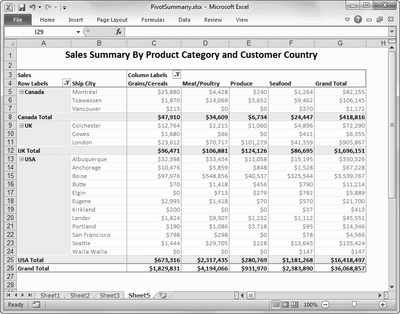
Figure 2. This spreadsheet summarizes a company’s total sales. The information is grouped based on where the company’s customers live, and it’s further divided according to product category. Summaries like these can help you spot profitable product categories and identify items popular in specific cities. This advanced example uses pivot tables, which are described in Chapter 22.
Although Microsoft is reluctant to admit it, most of Excel’s core features were completed nearly 10 years ago. So what has Microsoft been doing ever since? The answer, at least in part, is spending millions of dollars on usability tests, which are aimed at figuring out how easy—or difficult—a program is to use. In a typical usability test, Microsoft gathers a group of spreadsheet novices, watches them fumble around with the latest version of Excel, and then tweaks the program to make it more intuitive.
After producing Excel 2003, Microsoft finally decided that minor tune-ups couldn’t fix Excel’s overly complex, button-heavy toolbars. So they decided to undertake a radical redesign to create a user interface that actually makes sense. The centerpiece of this redesign is the super-toolbar called the ribbon.
Everything you’ll ever want to do in Excel—from picking a fancy background color to pulling information out of a database—is packed into the ribbon. To accommodate all these buttons without becoming an over-stuffed turkey, the ribbon uses tabs. Excel starts out with seven tabs in the ribbon. When you click one of these tabs, you see a whole new collection of buttons (Figure 3).
Note
Wondering what each tab holds? You’ll take a tab tour in Chapter 1 on A Tour of the Excel Window.
The ribbon is the best thing to hit the Excel scene in years. The ribbon makes it easier to find features and remember where they are, because each feature is grouped into a logically related tab. Even better, once you find the button you need, you can often find other, associated commands by looking at the section where the button is placed. In other words, the ribbon isn’t just a convenient tool—it’s also a great way to explore Excel.
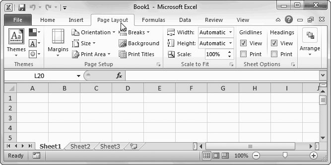
Figure 3. When you launch Excel, you start at the Home tab. But here’s what happens when you click the Page Layout tab. Now, you have a slew of options for tasks like adjusting paper size and making a decent printout. The buttons in a tab are grouped into smaller boxes for clearer organization.
The ribbon is full of craftsman-like detail. For example, when you hover over a button, you don’t see a paltry two- or three-word description in a yellow box. Instead, you see a friendly pop-up box with a complete mini-description and a shortcut that lets you trigger this command from the keyboard. Another nice detail is the way you can jump through the tabs at high velocity by positioning the mouse pointer over the ribbon and rolling the scroll wheel (if your mouse has a scroll wheel). And you’re sure to notice the way the ribbon rearranges itself when you change the size of the Excel window (see Figure 4).
If you’re an unredeemed keyboard lover, you’ll be happy to hear that you can trigger ribbon commands with the keyboard. The trick is using keyboard accelerators, a series of keystrokes that starts with the Alt key (the same key you used to use to get to a menu). When using a keyboard accelerator, you don’t hold down all the keys at the same time. (As you’ll soon see, some of these keystrokes contain so many letters that you’d be playing Finger Twister if you tried holding them all down simultaneously.) Instead, you hit the keys one after the other.
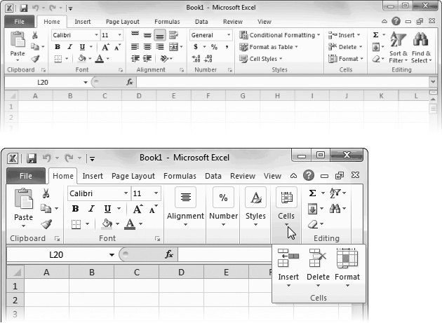
Figure 4. Top: A large Excel window gives you plenty of room to play. The ribbon uses the space effectively, making the most important buttons bigger. Bottom: When you shrink the Excel window, the ribbon rearranges its buttons and makes some smaller (by shrinking the button’s icon or leaving out the title). Shrink small enough, and you might run out of space for a section altogether. In that case, you get a single button (like the Number, Styles, and Cells sections in this example) for an entire section. Click this button and the missing commands appear in a drop-down panel.
The trick to using keyboard accelerators is to understand that once you hit the Alt key, there are two things you do, in this order:
Pick the ribbon tab you want.
Choose a command in that tab.
Before you can trigger a specific command, you must select the correct tab (even if it’s already displayed). Every accelerator requires at least two key presses after you hit the Alt key. You need even more if you need to dig through a submenu.
By now, this whole process probably seems hopelessly impractical. Are you really expected to memorize dozens of different accelerator key combinations?
Fortunately, Excel is ready to help you out with a feature called KeyTips. Here’s how it works. Once you press the Alt key, letters magically appear over every tab in the ribbon. Once you hit a key to pick a tab, letters appear over every button in that tab (Figure 5). You can then press the corresponding key to trigger the command (Figure 6).
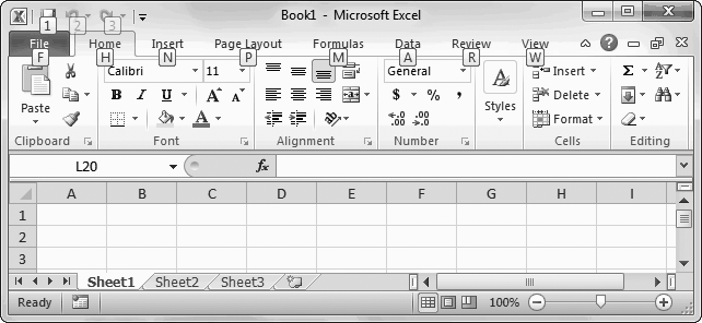
Figure 5. When you press Alt, Excel helps you out with KeyTips next to every tab, over the File menu, and over the buttons in the Quick Access toolbar. If you follow up with M (for the Formulas tab), you’ll see letters next to every command in that tab, as shown in Figure I-6.
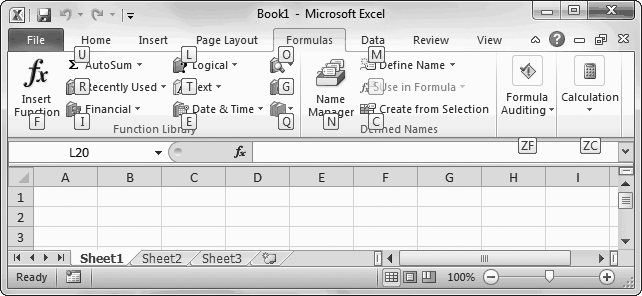
Figure 6. You can now follow up with F to trigger the Insert Function button, U to get to the AutoSum feature, and so on. Don’t bother trying to match letters with tab or button names—there are so many features packed into the ribbon that in many cases the letters don’t mean anything at all.
In some cases, a command might have two letters, in which case you need to press both keys, one after the other. (For example, the Find & Select button on the Home tab has the letters FD. To trigger it, press Alt, then H, then F, and then D.)
Tip
You can back out of KeyTips mode without triggering a command at any time by pressing the Alt key again.
There are other shortcut keys that don’t use the ribbon. These are key combinations that start with the Ctrl key. For example, Ctrl+C copies highlighted text and Ctrl+S saves your work. Usually, you find out about a shortcut key by hovering over a command with the mouse. For example, hover over the Paste button in the ribbon’s Home tab, and you see a tooltip that tells you its timesaving shortcut key is Ctrl+V. And if you’ve worked with a previous version of Excel, you’ll find that Excel 2010 keeps all of the same shortcut keys.
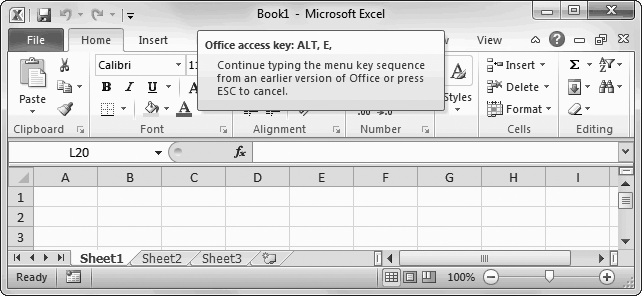
Figure 7. By pressing Alt+E, you’ve triggered the “imaginary” Edit menu from Excel 2003 and earlier versions. You can’t actually see it (because in Excel 2010 this menu doesn’t exist). However, the tooltip lets you know that Excel is paying attention. You can now complete your action by pressing the next key for the menu command you’re nostalgic for.
Excel 2010 doesn’t introduce anything earth-shattering as the ribbon. However, it does have another not-so-small change to the way the program operates. Instead of sending you to an ordinary menu to open files, create them, and print your work, it devotes the entire window to these tasks—once you switch into a mode called backstage view.
To switch to backstage view, click the File button that appears just to the left of the Home tab in the ribbon. (The name of this button is a nod to Excel 2003 and other older, more traditional Windows programs, which group many of these tasks together in a menu named File.) To get out of backstage view, just click File again or press the Esc key.
Backstage view is split into two parts. On the left is a narrow strip of different commands. You click one of these to show a page for a different task. Depending on what you click, Excel may show additional options and information on the right, as shown in Figure 8.
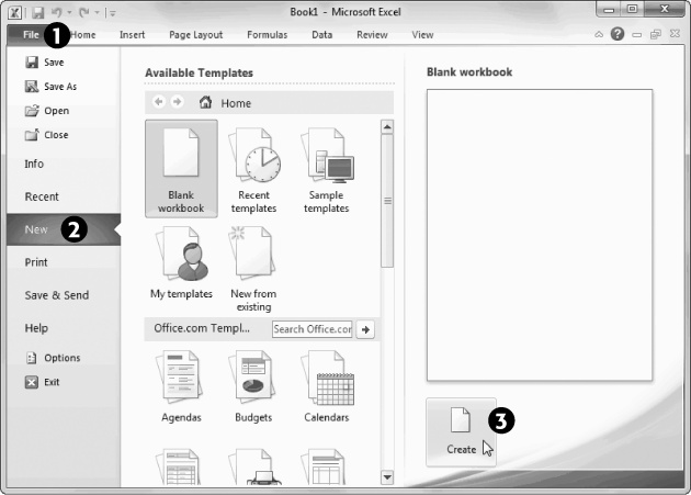
Figure 8. To create a new Excel workbook, start by clicking the File tab (1) and then the New command on the left (2). Excel uses its big backstage view to show you a slew of options. For a no-fuss blank workbook, just leave “Blank workbook” selected and click the Create button on the right (3). Or, if you want to get a head start with a premade template, choose one of the many other options underneath. (Chapter 16 tackles templates in detail.)
Here are some of the things you’ll do in Excel’s backstage view:
Work with files (creating, opening, closing, and saving them). You’ll do plenty of this in Chapter 1.
Print your work (Chapter 7) and send it off to other people by email (Chapter 25).
Prepare a workbook to be shared with other people. For example, you can check its compatibility with old versions of Excel (Chapter 1) and use document protection to prevent other people from changing your numbers (Chapter 24).
Configure how Excel behaves. Once you’re in backstage view, just click the Options command to get to the Excel Options dialog box, an all-in-one place for configuring Excel (Excel Options).
Keen eyes will have noticed the tiny bit of screen real estate on the right side of the Office button, just above the ribbon. It holds a series of tiny icons, like the toolbars in older versions of Excel (Figure 9). This is the Quick Access toolbar (or QAT, to Excel nerds).
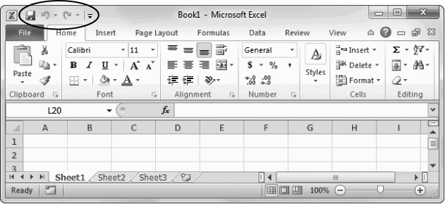
Figure 9. The Quick Access toolbar puts the Save, Undo, and Redo command right at your fingertips. These commands are singled out because most people use them more frequently than any other commands. But as you’ll learn in the Appendix, you can add anything you want here.
If the Quick Access toolbar were nothing but a specialized shortcut for three commands, it wouldn’t be worth the bother. However, the nifty thing about the Quick Access toolbar is that you can customize it. In other words, you can remove commands you don’t use and add your own favorites. The appendix of this book shows how.
Microsoft has deliberately kept the Quick Access toolbar very small. It’s designed to provide a carefully controlled outlet for those customization urges. Even if you go wild stocking the Quick Access toolbar with your own commands, the rest of the ribbon remains unchanged. (And that means a co-worker or spouse can still use your computer without suffering a migraine.)
As you’ve already learned, Excel 2010 isn’t nearly as radical as Excel 2007, which revamped the program’s main window and introduced the now-infamous ribbon. However, Excel 2010 still has its share of enhancements. Here are the most important:
Backstage view. Now Excel has a single go-to place for managing files. Whether you need to open an existing spreadsheet, create a new one, print your work, or tune up Excel options, Excel’s backstage view gives you a bit more breathing room. You’ll learn more about this mega-timesaver in Chapter 1.
Better AutoRecover. Excel has always had an emergency failsafe feature that preserves your work in the event of computer disaster (for example, a power failure). But now you can use the same feature to rescue your work after a personal blunder (for example, forgetting to save your work or suddenly realizing you deleted a critical piece of information 40 minutes ago). That’s because Excel 2010 stores a list of automatically backed-up files and lets you open them if you need to make an emergency recovery (AutoRecover).
Paste preview. Now you can see what the result of a copy-and-paste will be before you actually do it. It seems like a minor refinement, but when you’re using advanced paste options—for example, trying to decide whether to copy your numbers and their formatting—it’s a huge convenience. Fancy Pasting Tricks has more.
Sparklines. These miniature graphs are the hottest innovation in data display since the invention of the pie chart. They’re small (so they can fit into a single cell), but still big enough for you to see trends and summaries at a glance. If a full-fledged chart seems like overkill in your spreadsheet, a sparkline just might be what you’re looking for. Chapter 20 describes sparklines in detail.
Protected view. Do you live in fear of marauding Excel viruses corrupting your computer? Well, even if you don’t, you’ll be happy to know that Excel opens potentially dangerous spreadsheets in a carefully restricted window, ensuring they can’t get up to any trouble. Thanks to this change, you can open a spreadsheet straight from the Web or your email inbox, without worry. Protected View shows how it works.
Slicers. If you’ve ever run into Excel’s pivot tables, you know that they’re powerful but complicated. But life gets a bit easier with slicers (Slicers), a new feature that gives you a visual way to slice and dice your pivot table data, filtering it down to the details that interest you the most.
Easier ribbon customization. In Excel 2007, you couldn’t change the ribbon unless you mastered an intimidating extensibility model based on XML. Now, you just need a leisurely trip to the Customize Ribbon section of the Excel Options dialog box, where you can add, remove, and reorder Excel’s panoply of buttons to suit your personal preferences. The Appendix shows you how.
The Excel Web App. Wouldn’t it be cool to view your Excel spreadsheet in a web browser? And wouldn’t it be even better if you could edit it and share with other people? And wouldn’t it be just a little mind-blowing if you could use the Excel Web App to work on an Excel spreadsheet, even if you didn’t have Excel installed on your computer? For the first time, Excel 2010 makes these scenarios possible. You’ll get the scoop in Chapter 26.
Of course, this list is by no means complete. Excel 2010 is chock-full of refinements, tweaks, and tune-ups that make it easier to use than any previous version. You’ll learn all the best tricks throughout this book.
Despite the many improvements in software over the years, one feature hasn’t improved a bit: Microsoft’s documentation. In fact, with Office 2010, you get no printed user guide at all. To learn about the thousands of features included in this software collection, Microsoft expects you to read the online help.
Occasionally, the online help is actually helpful, like when you’re looking for a quick description explaining a mysterious new function. On the other hand, if you’re trying to learn how to, say, create an attractive chart, you’re stuck with terse and occasionally cryptic instructions.
The purpose of this book, then, is to serve as the manual that should have accompanied Excel 2010. In these pages, you’ll find step-by-step instructions and tips for using almost every Excel feature, including those you may not even know exist.
This book is divided into eight parts, each containing several chapters.
Part One: Worksheet Basics. In this part, you’ll get acquainted with Excel’s interface and learn the basic techniques for creating spreadsheets and entering and organizing data. You’ll also learn how to format your work to make it more presentable, and how to create sharp printouts.
Part Two: Formulas and Functions. This part introduces you to Excel’s most important feature—formulas. You’ll learn how to perform calculations ranging from the simple to the complex, and you’ll tackle specialized functions for dealing with all kinds of information, including scientific, statistical, business, and financial data.
Part Three: Organizing Your Information. The third part covers how to organize and find what’s in your spreadsheet. First, you’ll learn to search, sort, and filter large amounts of information by using tables. Next, you’ll see how to boil down complex tables with grouping and outlining. Finally, you’ll turn your perfected spreadsheets into reusable templates.
Part Four: Charts and Graphics. The fourth part introduces you to charting and graphics, two of Excel’s most popular features. You’ll learn about the wide range of different chart types available and when it makes sense to use each one. You’ll also find out how you can use pictures to add a little pizazz to your spreadsheets.
Part Five: Advanced Data Analysis. In this short part, you’ll tackle some of the more advanced features that people often overlook or misunderstand. You’ll see how to study different possibilities with scenarios, use goal seeking and the Solver add-in to calculate “backward” and fill in missing numbers, and create multi-layered summary reports with pivot tables.
Part Six: Sharing Data with the Rest of the World. The sixth part explores ways that you can share your spreadsheets with other people. You’ll learn how to collaborate with colleagues to revise a spreadsheet, without letting mistakes creep in or losing track of who did what. You’ll also learn how to copy Excel tables and charts into other programs (like Word) and how to use the Excel Web App to share and edit spreadsheet on the Web.
Part Seven: Programming Excel. This part presents a gentle introduction to the world of Excel programming, first by recording macros and then by using the full-featured VBA (Visual Basic for Applications) language, which lets you automate complex tasks.
Part Eight: Appendix. The end of this book wraps up with an appendix that shows how to customize the ribbon to get easy access to your favorite commands.
Throughout this book, you’ll find sentences like this one: “Choose Insert→Illustrations→Picture.” This a shorthand way of telling you how to find a feature in the Excel ribbon. It translates to the following instructions: “Click the Insert tab of the toolbar. On the tab, look for the Illustrations section. In the Illustrations box, click the Picture button.” Figure 10 shows the button you want.
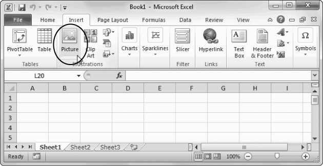
Figure 10. In this book, arrow notations help to simplify ribbon commands. For example, “Choose Insert→Illustrations→Picture” leads to the highlighted button shown here.
Note
As you saw back in Figure 4, the ribbon adapts itself to different screen sizes. Depending on the size of your Excel window, it’s possible that the button you need to click won’t include any text. Instead, it shows up as a small icon. In this situation, you can hover over the mystery button to see its name before deciding whether to click it.
There are some tabs that appear in the ribbon only when you’re working on specific tasks. For example, when you create a chart, a Chart Tools section appears with three new tabs (see Figure 11).
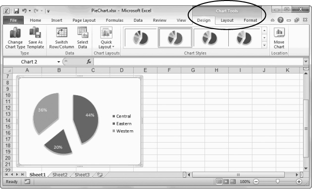
Figure 11. Excel doesn’t bother to show these three tabs unless you’re working on a chart, because it’s frustrating to look at a bunch of buttons you can’t use. This sort of tab, which appears only when needed, is called a contextual tab.
When dealing with contextual tabs, the instructions in this book always include the title of the tab section (it’s Chart Tools in Figure 11). Here’s an example: “Choose Chart Tools | Design→Type→Change Chart Type.” Notice that the first part of this instruction includes the tab section title (Chart Tools) and the tab name (Design), separated by the | character. That way, you can’t mistake the Chart Tools | Design tab for a Design tab in some other group of contextual tabs.
From time to time, you’ll encounter buttons in the ribbon that have short menus attached to them. Depending on the button, this menu might appear as soon as you click the button, or it might appear only if you click the button’s drop-down arrow, as shown in Figure 12.
When dealing with this sort of button, the last step of the instructions in this book tells you what to choose from the drop-down menu. For example, say you’re directed to “Home→Clipboard→Paste→Paste Special.” That tells you to select the Home tab, look for the Clipboard section, click the drop-down part of the Paste button (to reveal the menu with extra options), and then choose Paste Special from the menu.
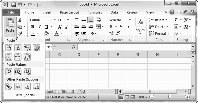
Figure 12. There are several options for pasting text from the clipboard. Click the top part of the Paste button to perform a plain-vanilla paste (with all the standard settings), or click the bottom part to see the menu of choices shown here.
Tip
Be on the lookout for drop-down arrows in the ribbon—they’re tricky at first. You need to click the arrow part of the button to see the full list of options. When you click the other part of the button, you don’t see the list. Instead, Excel fires off the standard command (the one Excel thinks is the most common choice) or the command you used most recently.
As powerful as the ribbon is, you can’t do everything using the buttons it provides. Sometimes you need to use a good ol'-fashioned dialog box. (A dialog box is a term used in the Windows world to describe a small window with a limited number of options. Usually, dialog boxes are designed for one task and aren’t resizable, although software companies like Microsoft break these rules all the time.)
There are two ways to get to a dialog box in Excel 2010. First, some ribbon buttons take you there straight away. For example, if you choose Home→Clipboard→Paste→Paste Special, you always get a dialog box. There’s no way around it.
The second way to get to a dialog box is through something called a dialog box launcher, which is just a nerdified name for the tiny square-with-arrow icon that sometimes appears in the bottom-right corner of a section of the ribbon. The easiest way to learn how to spot a dialog box launcher is to look at Figure 13.
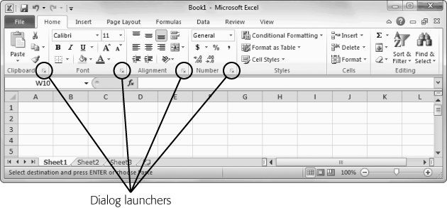
Figure 13. As you can see here, the Clipboard, Font, Alignment, and Number sections all have dialog box launchers. The Styles, Cells, and Editing sections don’t.
When you click a dialog box launcher, the related dialog box appears. For example, click the dialog box launcher for the Font section and you get a full Font dialog box that lets you scroll through all the typefaces on your computer, choose the size and color, and so on.
In this book, there’s no special code word that tells you to use a dialog box launcher. Instead, you’ll see an instruction like this: “To see more font options, look at the Home→Font section and click the dialog box launcher (the small icon in the bottom-right corner).” Now that you know what a dialog box launcher is, that makes perfect sense.
If you see an instruction that includes arrows but starts with the word File, it’s telling you to go to Excel’s backstage view. For example, the sentence “Choose File→New” means click the File button to switch to backstage view, then click the New command (which appears in the narrow list on the left). To take another look at backstage view and the list of commands it offers, jump back to Figure 8 on page 9.
There are also a couple of cases where you’ll still use the familiar Windows menu. One example is when you use the Visual Basic editor (in Chapter 29). In this case, the arrows refer to menu levels. For example the instruction “Choose File→Save” means “Click the File menu heading. Then, on the File menu, click the Save command.”
Every time you take your hand off the keyboard to move the mouse, you lose a few microseconds. That’s why many experienced computer fans use keystroke combinations instead of toolbars and menus wherever possible. Ctrl+S, for example, is a keyboard shortcut that saves your current work in Excel (and most other programs).
When you see a shortcut like Ctrl+S in this book, it’s telling you to hold down the Ctrl key and, while it’s down, press the letter S, and then release both keys. Similarly, the finger-tangling shortcut Ctrl+Alt+S means hold down Ctrl, and then press and hold Alt, and then press S (so that all three keys are held down at once).
As you read this book, you’ll see a number of examples that demonstrate Excel features and techniques for building good spreadsheets. Most of these examples are available as Excel workbook files in a separate download. Just surf to www.missingmanuals.com/cds and click the link for this book to visit a page where you can download a ZIP file that includes the examples, organized by chapter.
At http://www.missingmanuals.com, you’ll find news, articles, and updates to the books in the Missing Manual series.
But the website also offers corrections and updates to this book (to see them, click the book’s title, and then click Errata). In fact, you’re invited and encouraged to submit such corrections and updates yourself. In an effort to keep the book as up-to-date and accurate as possible, each time we print more copies of this book, we’ll make any confirmed corrections you’ve suggested. We’ll also note such changes on the website, so that you can mark important corrections in your own copy of the book.
In the meantime, we’d love to hear your own suggestions for new books in the Missing Manual series. There’s a place for that on the website, too, as well as a place to sign up for free email notification of new titles in the series.
Safari® Books Online is an on-demand digital library that lets you easily search over 7,500 technology and creative reference books and videos to find the answers you need quickly.
With a subscription, you can read any page and watch any video from our library online. Read books on your cellphone and mobile devices. Access new titles before they’re available for print, and get exclusive access to manuscripts in development and post feedback for the authors. Copy and paste code samples, organize your favorites, download chapters, bookmark key sections, create notes, print out pages, and benefit from tons of other time-saving features.
O’Reilly Media has uploaded this book to the Safari Books Online service. To have full digital access to this book and others on similar topics from O’Reilly and other publishers, sign up for free at http://my.safaribooksonline.com.
Get Excel 2010: The Missing Manual now with the O’Reilly learning platform.
O’Reilly members experience books, live events, courses curated by job role, and more from O’Reilly and nearly 200 top publishers.

