Data entry is the heart of Excel. If you can’t get data into your worksheet quickly and accurately, you can’t use the nifty tools at your disposal to analyze them. Excel does a lot of things right when it comes to data entry, but some things are downright peculiar. If you’ve ever had Excel correct your typing when you know what you entered was right, or turn a six-digit integer into a date, you know what I’m talking about.
The first part of this chapter shows you how to blow away Excel’s everyday data annoyances, from it’s habit of deleting leading zeros to correcting you obsessively. You’ll also encounter (and solve) annoyances when creating forms, importing data, cutting and pasting, navigating in and among worksheets, and more. Finally, we’ll focus on Excel’s handy data validation feature. With validation rules, you can limit the kind of data users can enter in cells. The rules can require values to fall into a specific range, or force the user to pick values from a list. This is a boon to managing data entry, but it can be a major annoyance to set up.
I can’t tell you how many times I’ve been happily entering data, only to have that blasted paperclip “helper” thing elbow its way onto the screen. By the time I get rid of it, I’ve lost track of what I’m doing and it takes me forever to get back in the groove. If that Office Assistant really were a live office assistant, I’d have had fired him years ago! How do I make it go away?
Clippy is one of the most-hated Office “innovations” in history. Microsoft had the good sense to turn off Clippy and his companion Office Assistant characters by default in Excel 2002 (the Office XP version) and in later versions.
In Excel 97, you can terminate Clippy permanently by opening the \Program Files\Microsoft Office\Office folderand renaming the Actors subfolder to something such as Old_Actors or Ha_ha_ha. Once Excel (and your other Office programs) can no longer find the Actors subfolder, Clippy will be unable to appear out of nowhere like a $1,000 bar tab.
If you’re using Office 2000 or XP, you can turn off Clippy by going to the Control Panel and using either the Add/Remove Programs applet or (depending on your operating system) the Add or Remove Programs applet. In Windows Me, 2000, or XP, click Microsoft Office in the Currently Installed Programs list and then click Change. Click the Add or Remove button, click the Office Tools item, click Office Assistant, and then click Not Available. Confirm your choices and you’re done. If you’re running Windows 98, click the Microsoft Office entry in the Install/Uninstall tab, click Add/Remove Program, and step through the wizard until you can change the Office Assistant’s setting to Not Available.
If you’re using Office 2003, you can turn off Clippy by going through the Add or Remove Programs control panel. In the Currently Installed Programs list, click Microsoft Office 2003 and then click Change. Select the Add or Remove option button on the first page of the wizard and click Next. Check the “Choose advanced customization of applications” box and click Next. Expand the Shared Office Features item, click Office Assistant, click Not Available, and then click Update.
Tip
Be forewarned that the Office Update wizard might ask for your Office installation CD to make these changes. You can avoid this request by installing every Office component to your hard disk.
There are several funny articles about giving Clippy the boot. You can find two of them at http://www.techsoc.com/clippyfired.htm and http://www.techsoc.com/clippynow.htm. For those with a darker sense of humor, you can find out how Clippy can help you to write one final letter at http://www.techsoc.com/clippycide.htm.
My company uses five-digit product codes, and some of them start with zero. My problem is that when I enter a product code with a leading zero, Excel deletes the zero. For example, Excel turns product 03182 into product 3182, which generates horrible errors in my macros, not to mention my inventory. How do I stop this behavior?
Unless you tell it differently, Excel expects you to enter numbers without leading zeroes. This can also be a problem with scientific numbers (e.g., 0.16 microns), which likewise often have leading zeros. Fortunately there is a way to convince Excel to let you enter values with leading zeros, by treating those values as a bit of text and not a number. Here’s how:
Select the cells that will contain numbers stored as text.
Right-click the cell and choose Format → Cells, then click the Number tab (as shown in Figure 1-1).
Click Text in the Category list and then click OK.
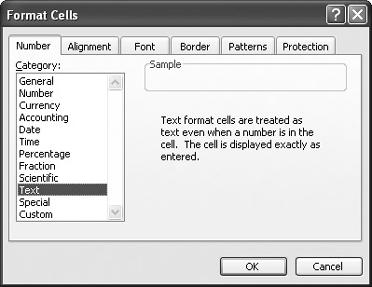
Figure 1-1. The Format Cells dialog box lets you tell Excel how to treat data entered or imported into your workbook.
You’ve changed the cells’ format from General (which expects a number, or something readily identifiable as text) to Text, which treats everything (even numbers) as if it’s the kind of alphanumeric text you’d find in a Word document.
You can use the same fix to prevent Excel from converting certain numbers (such as 100349 or 021264) into date/time format (a problem that’s described in more detail in Chapter 3). For instance, in the medical field, where privacy is of paramount importance, you might use case numbers such as these to track your patients. If you don’t want Excel to change these numbers to dates (Oct-3, 1949, in the first example), set the format of the cell to Text before you import or type in the case number.
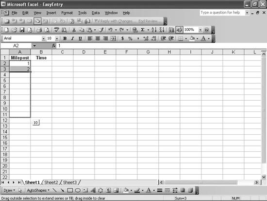
I’m so tired of entering regular sequences of data into cells. I mean, typing 1 in cell A1, then 2 in cell A2, then 3 in cell A3, then 4 in cell A4...up to 100 or 200. This isn’t a good use of my time! Isn’t there some way to extend a data series automatically so that I don’t get carpal tunnel typing row headings?
You can enter a data series quickly and easily by typing the first two numbers in the series in adjacent cells. Then select those cells and drag the fill handle (that black square that appears at the bottom-right corner of the selected range, as shown in Figure 1-2) until the desired value appears in the tool tip that floats along next to your cursor.
The first two numbers in the series determine the relationship between successive cells for the rest of the series. For example, typing 1 in cell A1 and 3 in cell A2 would result in a series extended as 5 in A3, 7 in A4, and so on. Typing 5 in cell A1 and 10 in cell A2 would result in a series extended as 15 in A3, 20 in A4, and so on.
But what if you type in a series that doesn’t have a regular progression? In that case, Excel will use linear regression to approximate future values in the series. This can be very cool. For instance, if you have 10 years of sales totals and want to see what the numbers will look like if sales continue on their current trend, you can select the cells and drag the fill handle to fill in projected future values.
There’s actually a lot more to entering data series in Excel than simple linear projections. You can get at the more advanced series entry tools by right-dragging the fill handle to display a shortcut menu where you can pick the type of growth you want the series data to exhibit. If you click Linear Trend, you get the same trends I described earlier. If you click Geometric Trend, however, you get a series in which each value increases exponentially (that is, the base value is squared). For example, in a linear series the series would begin 1, 2, 3, 4, while in a growth series it would begin 1, 2, 4, 8.
Tip
The growth series discussed here represents powers of 2. Excel recognizes that the first element is 20, the second is 21, the third is 22, and so on. If the first four elements of the series were 1, 4, 9, 16, Excel would extend the series as 25 (52), 36 (62), and so forth.
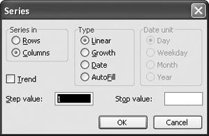
The final item on the shortcut menu you see when you right-drag the fill handle is Series. The Series dialog box (shown in Figure 1-3) has controls that let you determine how you want to extend the data series you’ve defined. For example, you can select a linear or geometric expansion. Clicking the AutoFill option is the equivalent of dragging the fill handle to extend a series. Checking the Trend box tells Excel to calculate the average percentage change in the selected cells and to put that value in the “Step value” box.
Can’t I just define the beginning and end values of a data series and specify the increment? Dragging is nice, but my bosses tell me how to create a series based on the first value, the last value, and the difference between each value.
At the bottom of the Series dialog box are the “Step value” and “Stop value” boxes, which let you create a data series beginning with a value defined in your worksheet. The step value is the difference between each item in the series, and the stop value is the last value in the series. For example, suppose you have the value 1 in cell A1. Select column A and choose Edit → Fill → Series. If you enter a step value of 2 and a stop value of 15, Excel will put values 1, 3, 5, 7, 9, 11, 13, and 15 in the range A1:A8. You need to select at least as many cells as you require for your series, though, or Excel will put values only in the cells you selected. For example, if you select cells A1:A3 and follow the procedure I just described, you’ll get only the values 1, 3, and 5 in those cells.
I hate my mouse. I always end up dragging stuff I don’t want to drag, or dropping it in the wrong cells, so even thinking about right-clicking this and right-dragging that fill handle thing gives me a panic attack. Isn’t there some way to create a data series without typing, clicking, and dragging?
Select options in the Series dialog box. You can create series based on dates and days without a bit of dragging. Excel knows about the following four sequences:
Sunday, Monday, Tuesday, Wednesday, Thursday, Friday, Saturday
Sun, Mon, Tue, Wed, Thu, Fri, Sat
January, February, March, April, May, June, July, August, September, October, November, December
Jan, Feb, Mar, Apr, May, Jun, Jul, Aug, Sep, Oct, Nov, Dec
Excel also will extend a time series for you. For example, extending a series that starts with 9:00 AM in cell A1 and 10:00 AM in cell A2 will place 11:00 AM in cell A3, 12:00 PM in cell A4, and so on. For information on creating your own series, see the next annoyance, "Create a Custom Fill Series.”
Tip
If you want to create a time series, you must place a space between the final zero in the time and the AM or PM designator. If you leave out that space, Excel will treat the cell’s contents as a General entry rather than a Time entry and won’t extend the series for you. 12:00 AM works. 12:00AM doesn’t.
Interesting things happen when you convert between a numeric series and a day or month series. For example, if you have the numbers 1 through 3 in cells A1:A3 and you right-drag the fill handle to cell A4 and click the Year option button, you’ll get a series that progresses like so: 1, 367, 732, 1097. Those increments are 366 (the number of days in a leap year—in this case, 2004) and 365 (the number of days in the years 2005 and 2006).
The stupid built-in data lists in Excel don’t have the values I want. Can I create my own fill series?
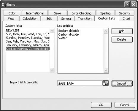
Yes, you can easily define a custom repeating sequence. For example, if you’re noting the amount of sodium chloride, carbon dioxide, and water produced by a chemical reaction, and you want to create a column with those labels repeating in the same order, you can type those values in cells A1:A3, select the cells, and drag the fill handle to repeat that sequence in every cell you drag the fill handle over. If you think you might use the sequence again for some reason, or if you want to use it for sorting your worksheet data, you can create a custom list. Here’s how:
Type the values you want in your custom list in a group of contiguous cells in a single column or row.
Select the cells containing your list and then select Tools → Options, and click the Custom Lists tab (shown in Figure 1-4).
Verify that the cell range you selected appears in the “Import list from cells” box. If it doesn’t, click the Collapse Dialog button (the tiny icon in the box at the far right), select the cells containing your list values, and then click the Expand Dialog button (in the box at the far right).
Click the Import button, and then click OK.
I’m adding data to a set of worksheets, and some of the matching cells on different sheets should contain the same data. For example, for the next three months I’m going to have five sales reps and a manager working from 9:00 a.m. until noon every day. I need to have a separate worksheet for each month (shown in Figure 1-5), and it’s a pain to have to reenter the data; isn’t there some way I can enter the data into cells in the range C2:C7 on all three sheets at the same time?
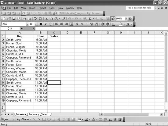
Entering data into the same cells on more than one worksheet at the same time sounds hard, but actually it’s pretty straightforward. Simply select the sheet tabs (found at the bottom lefthand corner of the Excel window) of the multiple worksheets in question and start typing. To select more than one worksheet at a time, use the standard Windows technique: Ctrl-click individual sheets; click one sheet tab and then Shift-click another to select that range of sheets; or right-click any sheet tab and click Select All Sheets to grab ‘em all.
I hate letting anyone mess around with my workbooks, but I’m in a time crunch and I need to let a co-worker enter data into one of my workbooks at the same time I work on it. Obviously, we can’t work on the same keyboard, but is there some way for both of us to edit the file at the same time?
If you use Excel 2000 or later, you can allow more than one user to edit a workbook simultaneously. First, put the workbook in a folder that other users can access. Then select Tools → Share Workbook, and check the “Allow changes by more than one user at the same time” box.
If you want to restrict who can open your shared workbook, follow these steps instead:
Choose Tools → Protection → Protect and Share Workbook, and check the “Sharing with track changes” box.
Type a password in the “Password (optional)” box.
Click OK.
Now no one can open the workbook unless you tell him the password.
I need to enter long paragraphs of text in some of the cells in my worksheet, and it would be great to start with a short headline on a separate line at the top. But every time I press Enter to separate the headline from the main text entry, Excel just takes me to a new cell. How in the world do I add a carriage return, line break, or whatever you call it? It’s driving me crazy!
I work for a multinational manufacturing company, and although I work exclusively in English, I do occasionally have to type a name in a foreign alphabet. My boss insists that I use the characters from the original language (Danish, German, and French are common), but I don’t know how to insert those letters, or other symbols, into my worksheet cells. Help!
In Excel 2002 and later, you can choose Insert → Symbol to display the “Symbol dialog” box, which lets you pick the symbol you want to insert. Just click the Insert button after you select your symbol. In Excel 97 and 2000, you must use Windows’ Character Map helper application to find the available symbols. To run Character Map in Windows XP, Me, or 98 select Start → Programs → Accessories → System Tools → Character Map. Once in Character Map, select the appropriate font, double-click the desired character (which copies it to the Clipboard), and then paste the character into your cell.
Excel is unshakably convinced that I don’t know how to spell. But Excel is wrong! I work for a company with an internal project code-named “ADN.” Go ahead; try typing that name into a cell. I’ll wait for you.
Excel changed it to “AND,” didn’t it? And you had to backspace over the code name and retype it, didn’t you? Drives me nuts. How do I make that stop happening?
You’ve got an overactive AutoCorrect feature. And although you should be grateful for all the times it’s prevented you from typing “teh” instead of “the,” it’s still a pain when it changes something you know is perfectly fine the way you typed it.
Tip
If Excel changes a word you type, you can press Ctrl-Z to undo the change—but only as long as you pressed the spacebar after you typed the word Excel corrected. If you press either the Tab key or the Enter key, Excel makes the change and then shifts its focus to the next active cell. That means that when you press Ctrl-Z, Excel erases the last change you made in the cell you just edited.
You can turn off AutoCorrect entirely by selecting Tools → AutoCorrect Options and unchecking the “Replace text as you type” box on the AutoCorrect tab page of the dialog box (shown in Figure 1-6).
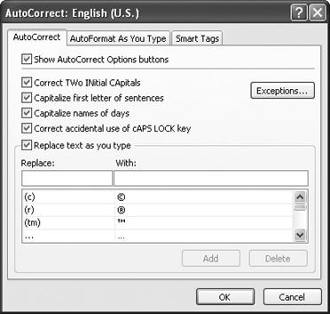
Figure 1-6. Stand up for what you know is right! Sometimes AutoCorrect requires a bit of manual correction.
If you want to modify only some of AutoCorrect’s behavior, you can uncheck the various boxes on this tab so that Excel won’t correct words starting with two or more capital letters, sentences (or what appear to be sentences) starting with a lowercase letter, lowercase day names, and the dreaded iNVERTED cAPS lOCK kEY. You even can define your own AutoCorrect entries by typing the term to be replaced in the Replace box, typing the term to replace it with in the With box, and clicking the Add button. By the same token, you can define exceptions to the initial-caps and first-letter rules by clicking the Exceptions button and filling in your exceptions in the dialog box that appears. Plus, you can delete individual AutoCorrect entries, such as the ADN/AND replacement you complained about, by selecting the entry from the list presented and clicking the Delete button.
If you type a URL in a cell, it automatically becomes a hyperlink, which is usually exactly what I don’t want to happen. How do I stop this?
Excel 97 doesn’t automatically format a URL as a hyperlink, so you’re in luck. In Excel 2000, there’s no way to keep Excel from formatting a URL as a hyperlink, but you can press Ctrl-Z right after it happens to remove the formatting. If you don’t catch it then, you also can click the cell and choose Insert → Hyperlink → Remove Hyperlink. For Excel 2002 or later versions, which do default to hyperlink formatting, you can stop Excel from transforming a URL or file path into a clickable link by adjusting the AutoCorrect function. Choose Tools → AutoCorrect Options, click the AutoFormat As You Type tab, and uncheck the “Internet and network paths with hyperlinks” box.
Get Excel Annoyances now with the O’Reilly learning platform.
O’Reilly members experience books, live events, courses curated by job role, and more from O’Reilly and nearly 200 top publishers.

