Excel Annoyances

CUT-AND-PASTE ANNOYANCES

PUT MORE THAN ONE ITEM ON THE CLIPBOARD

The Annoyance:

I frequently want to copy items from one workbook into another—or even into another application—and it’s tedious having to copy each cell, object, or image one by one, open the other document, paste what I copied, and then go back to my workbook and repeat. Can’t I collect what I cut or copy into a single intermediate location and then paste whatever I like?

The Fix:

It is possible to collect items you cut and copy in Excel into a single location, but how you do it changes drastically from version to version. In Excel 97, you’ll have to create a separate workbook or worksheet, and paste your collection in there. It’s a pain, but it works. Be sure to keep an eye on your workbook’s size so that it doesn’t slow down your system. I use 1MB as a guideline for when it’s time to create a new “holding tank,” but if you’re running an older system with less memory, you might want to set this limit at 500KB.

Microsoft introduced the Office Clipboard in Office 2000, and it’s been part of the suite ever since. The Office Clipboard keeps track of the last set of items you cut or copied (12 in Office 2000, 24 in XP and 2003) and makes them available to paste in any Office application, individually or all together. What’s even more interesting is that any items you cut or copy in one version of Office are available in other versions of Office that are open. At one point I had Word 2003 and Excel 2000, 2002, and 2003 running at the same time—and each program had the same three cut-and-copied items available in its Office Clipboard.

To use the Clipboard in Excel 2000, follow these steps:

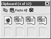
1. Choose View → Toolbars → Clipboard to display the Office 2000 Clipboard (shown in Figure 1-8).

   

   Figure 1-8. Paste-o-rama. With Office’s enhanced clipboard, you can cut and paste multiple selections at once.

2. Follow any of these steps to use the Clipboard:

   • Click an item and click Paste to paste that item into your worksheet.

   • Click Paste All to paste every item in the Clipboard into your worksheet.

   • Click Clear All to empty the Clipboard.

In Excel 2002 and Excel 2003, follow these steps to use the Clipboard:

1. Choose View → Task Pane.

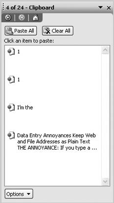
2. Click the Other Task Panes down arrow and click Clipboard to display the Clipboard task pane (the Excel 2003 version is shown in Figure 1-9).

   

   Figure 1-9. The Office Clipboard is implemented as a task pane in Excel 2002 and 2003.

3. Follow any of these steps to use the Clipboard:

   • Click an item to paste it into your worksheet.

   • Click Paste All to paste every item in the Clipboard into your worksheet.

   • Click Clear All to empty every item in the Clipboard.

   • To delete individual items, hover the mouse pointer over an item, click the down arrow that appears next to it, and choose Delete to remove it.

PREVENT THE OFFICE CLIPBOARD FROM APPEARING

The Annoyance:

I’m using Excel 2002, and whenever I cut or copy something, the Office Clipboard appears. It’s driving me crazy. How can I send it away?

The Fix:

The Clipboard toolbar won’t appear by itself in Excel 2000. If you’ve enabled it and you want it to go away, just right-click an empty spot on any toolbar and uncheck Clipboard. However, the Clipboard task pane can (and often does) appear by itself in Excel 2002 and 2003 when you copy or cut something. To keep it from appearing, follow these steps:

1. Choose View → Task Pane.

2. Unless Clipboard is already there, click the Other Task Panes down arrow at the top of the task pane and click Clipboard.

3. Click the Options button at the bottom of the pane, and uncheck the Show Office Clipboard Automatically box.

CONTROL PASTED CELL FORMATS

The Annoyance:

When I paste cells from one location to another, they keep their original formatting, which doesn’t always fit in with the cells around their new location. Is there a quick way to change the pasted cells’ format to that of their neighboring cells?

The Fix:

In Excel 97 or 2000, you can use the Format Painter to copy an existing format from one group of cells to another. Just click the cell with the format you want to copy, click the Format Painter button on the Standard toolbar (look for the little paintbrush), select the cells where you want to apply the format, and release the mouse button, and the format is applied. In Excel 2002 or 2003, when you paste something into a cell, the Paste Options button appears at the bottom right corner of the cells you pasted. Click it and select the Match Destination Formatting radio button to make the pasted cells take on the formatting of their new neighbors.

INSERT OR DELETE SINGLE CELLS

The Annoyance:

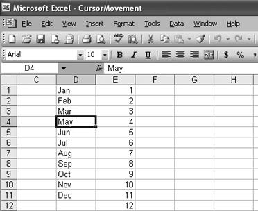
It’s easy enough to insert a row or column into a worksheet by right-clicking the column or row header and choosing Insert, but sometimes I need to insert just a single cell. In one worksheet, I typed in the sales data correctly, except that I left out the data that was supposed to go into cell D4 (see Figure 1-10). I could just cut and paste the data, but isn’t there a quick way to add a new cell at the D4 spot? And can I get rid of an extra cell?

Figure 1-10. All this worksheet needs is a new cell at D4.

The Fix:

Follow these steps to insert a cell into a worksheet:

1. Select a cell where you want a new, blank cell inserted.

2. Choose Insert → Cells, which displays the Insert dialog box.

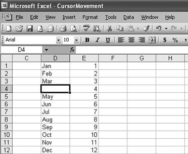
3. Depending on what you want to do, click the “Shift cells right” or “Shift cells down” radio button and click the OK button. You can see the result of clicking “Shift cells down” in Figure 1-11. The existing cell (holding “May”) is pushed down, and a new blank cell takes its place.

To insert multiple cells, simply select cells where you want new, blank cells inserted.

Figure 1-11. Make a new cell appear right where you need it.

To delete a cell or cells, follow these steps:

1. Select the cell or cells you want to delete.

2. Choose Edit → Delete.

3. Click the “Shift cells left” or “Shift cells up” radio button and click the OK button.

Tip

The cells don’t have to be in the same row or column, or even next to each other. Hold down the Ctrl key, click the desired cells, and then select Edit → Delete.

TRANSPOSE ROWS AND COLUMNS

The Annoyance:

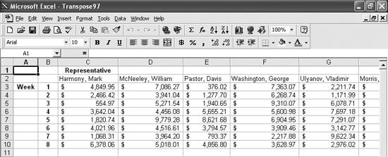
My boss told me to enter the weekly sales totals for all the representatives in our dealership, but for some reason she wants the reps’ names to appear as column headings and the week numbers as row headings. (A cut-down version of the worksheet appears in Figure 1-12.) Fine! Whatever she wants. But after the names started spilling off the right edge of the screen, she changed her mind and told me to make the rows into columns and the columns into rows. Is there any way to pull this off without cutting and pasting until my hand fall off?

Figure 1-12. Enter data with the wrong row/column orientation? There’s a way to flip ‘em.

The Fix:

Transposing rows and columns in a data selection isn’t too crazy. Just follow these steps:

1. Select the data you want to transpose, including all of the heading rows and columns, and the data itself, and choose Edit → Copy.

2. Click a cell outside the range you copied and choose Edit → Paste Special.

3. In the Paste Special dialog box check the Transpose box at the lower right and then click OK.

4. Select the original, untransposed block of data, including all the heading rows and columns, as well as the data, and choose Edit → Clear → All.

5. Select the data you just pasted and choose Edit → Cut.

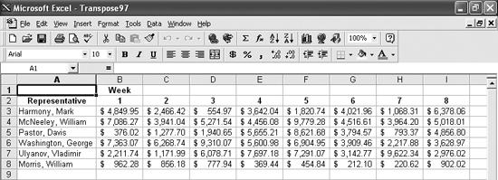
6. Click the cell at the top left corner of the range where you want the pasted data to appear and choose Edit → Paste. The result appears in Figure 1-13.

Tip

Formats don’t transpose well. Remove borders, cell fill colors, and so on, from the cells you plan to transpose, and reapply them after the final paste.

Figure 1-13. Don’t reenter the data—transpose it!

CHANGE THE DEFAULT SAVE LOCATION

The Annoyance:

I hate the fact that when I try to save an Excel document, it always tries to save it first in the My Documents folder. I usually want to save it somewhere else. Any ideas?

The Fix:

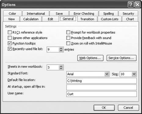
Instead of specifying the destination folder you want every time you save, just tell Excel what the default save folder should be. Choose Tools → Options and click the General tab shown in Figure 1-14. In the “Default file location” field, enter the path of your preferred save folder (such as C:\Reports\2004), click the OK button, and you’re good to go.

Figure 1-14. Use the controls on the General options page to change your default directory.