Excel Annoyances

CONDITIONAL FORMATTING ANNOYANCES

CHANGE CELL FORMATTING BASED ON THE CELL’S VALUE

The Annoyance:

I’m a commercial gardener and I use Excel to track the temperature in my greenhouses. I want to automatically flag any hours during which the temperature is less than 75 degrees by displaying that cell’s value in red text. How do I do it?

The Fix:

Conditional formatting is one of Excel’s handiest features. To change a cell’s formatting based on its contents, follow these steps:

1. Select the cells you want to format and choose Format → Conditional Formatting to display the Conditional Formatting dialog box, shown in Figure 2-1.

   

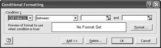
   Figure 2-1. Use the Conditional Formatting dialog box to change how your data looks based on its value.

2. Open the second drop-down menu and choose the comparison operator (between, less than, greater than, or equal to) you want to use to evaluate your data. Then type the associated values (the values the data is between, less than, greater than, or equal to) in the third and fourth boxes. (The fourth box doesn’t always appear; it depends on the Boolean operator you pick.) For this example, select “Less than” from the second drop-down menu, and in the box to the right, type in the value 75.

3. Click the Format button to tell Excel how it should format cells with values of less than 75. You can specify color, font style, underline, and strikethrough. Click OK ...