Excel Scientific and Engineering Cookbook

Chapter 1. Using Excel

Introduction

This chapter is necessarily basic and is intended for readers new to Excel or with little Excel experience. Experienced users may skip this chapter without loss of continuity. The aim of this chapter is to get you acquainted with Excel’s interface and the main features and capabilities that we’ll use throughout the remainder of this book. I’m also going to show you several techniques that will help you create presentable spreadsheets and allow you to work efficiently in Excel. The techniques and features summarized in this chapter will be put to use in the recipes throughout the remainder of this book.

1.1. Navigating the Interface

Problem

You’ve never used Excel before and don’t know where to start.

Solution

Start Excel and begin poking around the interface to become familiar with it.

Discussion

This solution sounds simple and it is. I believe there’s no better way to learn something on the computer than to just start exploring and experimenting. Don’t worry about breaking anything. The worst you can do is create a nonsensical spreadsheet—in which case, you can exit Excel without saving anything and start over fresh. I have a four-year-old daughter who loves playing around in Excel because of the paperclip office assistant. If she can’t ruin anything with all her random clicking and typing, then I think you’re in good shape to do some purposeful exploring. That said, I won’t just throw you to the wolves, but will point you in the right direction to begin your journey.

Excel is just like any other standard Windows application: it consists of a multiple-document interface main window containing a main menu bar, toolbars, and a status bar.

Tip

A multiple-document interface main window is just a window that acts as a container for several of the same type of files, so to speak. For example, in Excel you can have more than one spreadsheet open at once and switch between them. Word is another example; you can have many different Word documents open at once and switch between them as desired. By contrast, an application based on a single-document interface window is one that allows you to open up and work on only one file at a time. Many specialized programs are based on this paradigm.

Figure 1-1 shows a screenshot of Excel as installed on my computer. You’ll notice that it looks like any other Windows application, with one distinct difference.

Figure 1-1. Excel’s main window

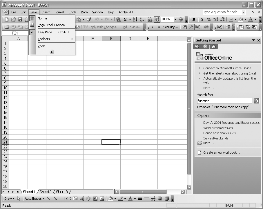
In addition to the standard menu bar, toolbars, and status bar, the window contains a large grid of cells . These cells are arranged in an organized matrix, with letters identifying columns and numbers identifying rows. This is the spreadsheet. Notice that there are a few tabs toward the bottom of the spreadsheet labeled Sheet 1, Sheet 2, and Sheet 3. By default, Excel starts with a blank workbook . A workbook contains multiple sheets, which can be linked together. You can add or remove spreadsheets from a workbook, rename the sheets, put data and formulas on one sheet and refer to them from another sheet, and so on. We’ll explore the details of working with spreadsheets and workbooks throughout the remainder of this book. For now, let’s continue getting acquainted with the window itself.

Main menu bar

The main menu bar gives you access to all of Excel’s features and functionality. Excel’s main menu bar contains the following menus:

File: Access the usual file operations such as open, save, print, and exit.
Edit: Access the standard cut, copy, paste, find, replace, and other operations.
View: Customize Excel’s appearance by changing options such as page layout, zoom, toolbars, status bar, and task pane.
Insert: Add various spreadsheet elements such as cells, rows, and columns, as well as other objects such as notes, comments, and pictures.
Format: Customize the formatting of text, cells, rows, columns, and other aspects of your spreadsheets.
Tools: Access various useful tools including spelling tools, change tracking, formula auditing, and a host of useful analysis tools such as goal seek, solver, and data analysis tools. The tools menu also provides access to the Customize and Options windows, allowing you to tailor Excel to your specific needs and preferences.
Data: Access various data management tools such as sorting, validation, and tables.
Window: Manage Excel’s windows by using features such as arranging windows and splitting panes.
Help: Access Excel’s built-in help system.

These nine menus comprise the standard menus built into Excel. I encourage you to click through these menus in your version of Excel to familiarize yourself with them a little. We’re going to use these menus a great deal throughout the remainder of this book.

Take another look at Figure 1-1 and notice that my version of Excel has one more menu option in addition to the nine just summarized. In my case, I have Adobe PDF converter installed, so a custom menu option for it appears in Excel’s main menu bar after the standard menus. (Such custom menus will not appear on your version of Excel unless you’ve installed third-party software that adds them.) I should mention that you can also add your own menus using techniques that we’ll discuss in other recipes throughout this book.

As with most standard Windows programs, you can access the menu using the mouse or the keyboard. Accessing the menu with the mouse is, of course, as simple as pointing and clicking. Notice in Figure 1-1 that the View menu is currently visible. Also notice the little down arrow icon at the bottom of the menu. Whenever you see this icon on a menu, it means there are more menu items available to you, but they are hidden. By default, MS Office applications hide less frequently used menu items from view, showing only your most frequently used items in an effort to simplify the menus. If you click the down arrow icon, the full menu will appear. I personally don’t like this feature and prefer to see the menus in their entirety all the time.

You can change this behavior by going to the Tools → Customize... menu and clicking the Options tab (see Figure 1-2).

Figure 1-2. Customize window

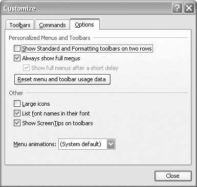
On the Options tab you’ll see a checkbox labeled “Always show full menus.” If you check that checkbox, full menus will be shown all the time. Otherwise, you’ll get the abbreviated menus, in which case you can select an option to show the full menus after a short delay. Press the Close button to save your changes and get rid of this window.

There are two ways to access menu items with the keyboard. The first way involves using the Alt key on your keyboard to set input focus on the main menu bar. In Excel, or any other Windows application for that matter, press the Alt key and you will notice that the first menu on the main menu bar gets highlighted. This means the menu has focus. Also notice that each menu—File, Edit, View, and so on—has one letter underlined. The underlined characters are called accelerator characters. After pressing the Alt key and giving focus to the main menu bar, you can press a key corresponding to one of those accelerator characters to open the corresponding menu. For example, the key sequence Alt-V will open the View menu, as shown in Figure 1-1.

You’ll notice each menu item in the View menu also contains an accelerator character. If you now press the key corresponding to one of these accelerators, you’ll activate the corresponding menu item. For example, the key sequence Alt-V-Z will activate the Zoom menu item, opening a new window that allows you to customize the zoom level of your spreadsheet. The zoom feature is helpful for those of us whose eyesight needs a little help.

The second way to access menu items from the keyboard involves the use of shortcut keys . Take another look at the View menu shown in Figure 1-1. Notice the Task Pane menu item has a key combination denoted to the right. In this case the key combination is Ctrl-F1 . This is the shortcut key combination to activate the Task Pane menu item. (This applies to Excel 2003. Earlier versions may not have this shortcut.) So, if you press and hold the Ctrl key and then press the F1 key (while still holding the Ctrl key down), you’ll activate the Task Pane menu item. When you execute this key combination, the task pane on the right side of the window will disappear. If you execute this shortcut again, the task pane will reappear. (We’ll come back to the task pane in a moment.)

Both of these keyboard techniques are designed to speed up your productivity by providing quick access to Excel’s functionality: you don’t have to keep taking your hand off the keyboard to navigate with the mouse. These quick access features are not unique to Excel and, in fact, are standard Windows interface features. Most well-designed Windows applications provide one or both of these features.

Task pane

I’ve already mentioned the task pane in the context of accessing menus using shortcuts (i.e., toggling the task pane’s visibility by using Ctrl-F1); however, I haven’t mentioned what the task pane actually does. The task pane provides another portal to features included in Excel, giving you access to Excel’s built-in and online help systems, a searchable dictionary and other reference material, and various spreadsheet templates. With Excel open as shown in Figure 1-1, click the little down arrow icon located to the right of the Getting Started title on the task pane to view the various tools available to you.

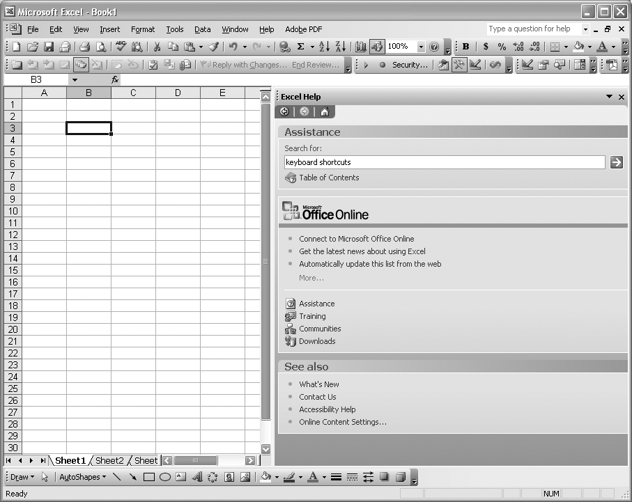
The one I find most useful is the Help tool. The Help tool is easy to use and provides access to both built-in and online sources of documentation on Excel . If you click the Help option, you’ll be presented with a text box at the top of the pane that allows you to type in search terms for topics.

For example, if you type in keyboard shortcuts, the task pane will switch to the Search Results view, displaying a list of topics related to your search terms. In my case, the topic Keyboard Shortcuts is at the top of the list. Find this in your version and click it. Upon doing so, you’ll be presented with a new help window showing a list of topics specifically related to keyboard shortcuts.

Tip

Excel has keyboard shortcuts for many features in addition to the menu shortcuts we discussed earlier. The help documentation describes all of those available to you and is a convenient reference for learning all sorts of useful shortcuts to help you work more efficiently. I encourage you to explore this documentation.

While the task pane does provide convenient access to some useful features, I find it sometimes gets in the way of my spreadsheet. So, when I’m not using it, I Ctrl-F1 it away or reduce its width by clicking and dragging the task pane’s left edge over toward the right, making more space for the spreadsheet.

Toolbars

Referring back to Figure 1-1, or your version of Excel if you have it open now, you’ll notice that the Excel window contains many toolbars and tool buttons. These are standard, dockable toolbars that provide yet another means to access Excel’s features. Many of the toolbars duplicate menu functionality, giving you another way of selecting menus; other toolbars provide access to features buried in various dialog boxes or windows that are themselves accessible from the menu or other toolbars. These toolbars are provided for convenience and it’s up to you to develop your own preferences, i.e., whether you prefer navigating the menu, using shortcut keys, or clicking tool buttons. I do all three.

You may have noticed that the toolbars in my version of Excel, shown in Figure 1-1, are different from those shown in your version of Excel. Certain toolbars that I use frequently are visible, while others are hidden. You can customize your toolbars to your liking. To do so, open the View menu and select the Toolbars submenu. This will display a list of toolbars available to you for display. The ones shown with checkmarks to their left are visible. You may select whichever ones you’d like to show or hide.

You can also customize the toolbars by using the Customize window shown in Figure 1-2. To activate this window, select Tools → Customize.... Select the Toolbars tab to display a list of available toolbars that you can show or hide.

Tip

The Commands tab in the Customize window allows you to further customize your toolbars. Using the Commands tool, you can select specific commands and then drag-and-drop a button corresponding to each command onto Excel’s toolbar area. This allows you to tailor your toolbars to contain only those command buttons you use most frequently, without cluttering your window with rarely used buttons.

Toolbars in Excel are dockable. This means you can drag them around to rearrange them. To do so, click (and hold) the four dots located to the left of a toolbar and drag it around. You can rearrange all your toolbars in this manner, placing some at the top of the window (below the main menu bar), some toward the bottom of the window (above the status bar), and some to the left or right of the window.

1.2. Entering Data

Problem

You’ve familiarized yourself with Excel’s layout and now you’re ready to enter data into a spreadsheet but don’t know how.

Solution

Select a cell in the spreadsheet and starting typing. Press Enter when done.

Discussion

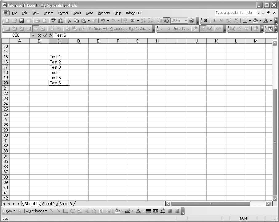
When you select a cell in a spreadsheet, it becomes highlighted with a thick black border, as shown in Figure 1-3. In that figure the cell in row 3 and column B is the selected cell. Notice the row and column headings of the currently selected cell are highlighted. Once a cell is selected in this manner, you can simply start typing on the keyboard to insert text in the cell. Press Enter when you are finished and notice that the cell below the one within which you entered text is now automatically selected. This allows you to type and enter text in a column of cells rapidly, without having to select the next cell using the mouse.

Figure 1-3. Excel Help task pane

Upon entering text, you can also press the Tab key to commit your entry and move the cell selection to the next cell to the right. Alternatively, you can use the arrow keys on your keyboard to commit an entry and move to any cell adjacent to the cell within which you’ve entered text. Of course you can always use the mouse to click on a cell, selecting it for input; however, doing this may slow you down if you are trying to enter text in a contiguous group of cells, since you’ll have to remove your hands from the keyboard very often.

You can also enter text into a cell using the formula bar (located just above the spreadsheet grid and just below the toolbars), as shown in Figure 1-4. The formula bar has an f _x icon, adjacent to a long white rectangular area.

Click anywhere in the white rectangular area of the formula bar to give it the input focus and then start typing. Your text will appear in both the formula bar and the currently selected cell. To commit the entry, press the Enter key or press the green checkmark icon on the formula bar. To cancel your entry, press the red × icon or press the Esc key on your keyboard.

Figure 1-4. Using the formula bar

Let’s say you want to make changes to some text already entered in a cell. To make changes to a cell entry, select the cell with the mouse or use the arrow keys to navigate the grid and then press the F2 shortcut key to put the cell in edit mode, allowing you to edit the contents of the cell. Alternatively, double-clicking on a cell will automatically select it and put it in edit mode. Finally, you can always select a cell and simply start typing and press Enter to completely overwrite the contents of the cell.

1.3. Setting Cell Data Types

Problem

You’ve learned how to enter text from the previous recipe, but now you want to enter data other than text (e.g., numbers, dates, and currency).

Solution

Enter the data just as you would text and let Excel automatically figure out its type, or use the Format → Cells... menu to open a dialog box allowing you to manually format the data type for a cell.

Discussion

In the previous recipe, I had you simply enter text in cells. Whether you entered a word or a number, Excel automatically figured out what type of data you entered. In general, input starting with letters is automatically interpreted as text, and input starting with numbers is automatically interpreted as numeric. There are some special cases worth noting here. Preceding any string of characters—numbers or letters—with the ' symbol forces Excel to interpret the data as text. Preceding a string of numbers with the $ symbol forces Excel to interpret the data as currency. Using E (or e) while entering a number in scientific notation forces Excel to interpret the string as a number in scientific notation. Entering numbers with dashes between them will cause Excel to interpret the number as a date. I encourage you to try entering various types of data like those I describe here to see how Excel handles the data. In some cases you’ll notice that Excel will reformat your data a little. For example, if you type 1.2345e3 in a cell, it will appear as 1.23E+3 in the cell and 1234.56 in the formula bar (when the cell is selected).

In general, Excel is pretty smart about interpreting the data type you intend; however, sometimes it does need a little help. Also, sometimes you may want to change the format of the data to give it an appearance other than the default appearance assigned to it by Excel. In these cases you can manually specify the type and format of data contained in cells by accessing the Format Cells dialog box . You can do so by selecting Format → Cells... from the menu or by using the shortcut key combination, Ctrl-1.

Figure 1-5 shows the Format Cells dialog box. Notice here I had a cell selected that contained the entry 1.2345e3, which appears in the Sample area of the dialog box. This allows you to preview the results while making format changes.

I find that one of the most common uses of formatting tasks is specifying the number of decimal places to show for numbers. You can specify the number of decimal places to show by entering a value in the “Decimal places” field. Changing this setting is a format change only; it does not change the data itself. For example, if you enter 123.45678 in a cell and set the number of decimal places to 3, the cell will show 123.457 but the actual number is still stored as 123.45678, as can be seen in the formula bar when the cell is selected.

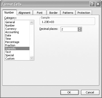
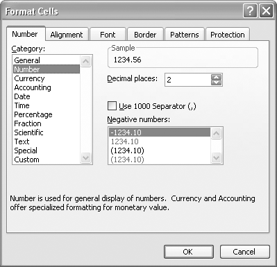
You can also select one of the categories shown in the Format Cells dialog box to set the type of data. If you click each category in the list, a short description and other formatting options will appear in the Format Cells dialog box. For example, if you select the Number category, the Format Cells dialog box will appear (see Figure 1-6).

The new formatting options appear on the right side of the dialog box, just under the “Decimal places” setting.

Format changes affect the currently selected cell and remain in effect until you change the format. If you set a cell to display Currency and then enter a new value in that cell, it will also be interpreted as currency.

Figure 1-5. Format cells dialog box

Figure 1-6. Format Cells with the Number category selected

You need not always use the Format Cells dialog box to change cell formatting. Some of these formatting operations have been assigned to toolbar buttons for convenience. Take a look at Figure 1-7 and notice the toolbar buttons that I highlighted. These specific buttons allow you to change some cell format properties with the click of a button.

Figure 1-7. Cell format toolbar

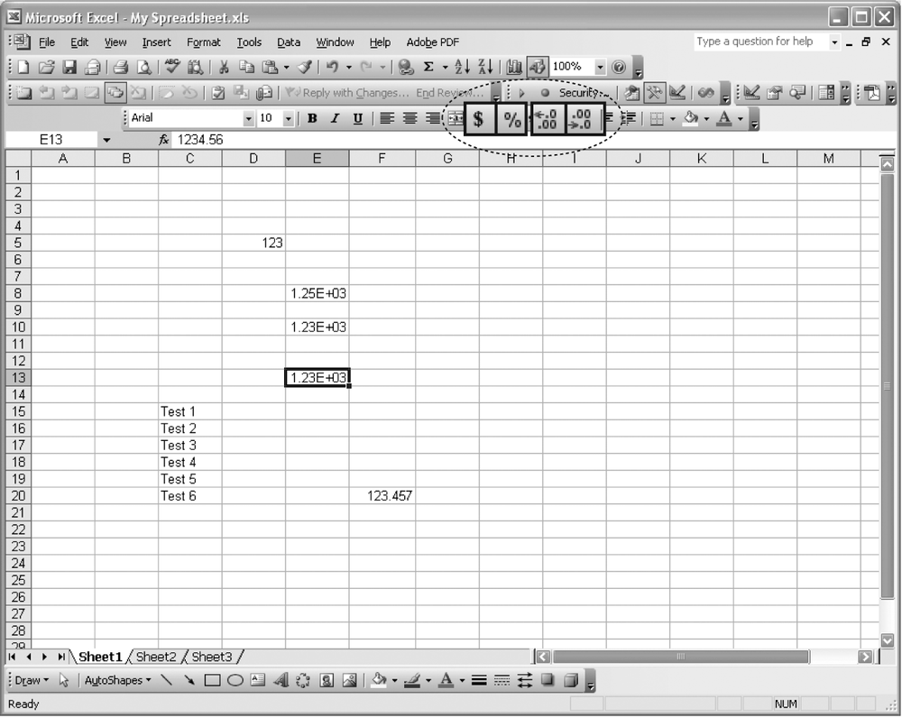
The $ button changes the cell format to currency while the % button changes the cell format to percentage; e.g., if you enter 0.38, it will show up as 38%. The two other highlighted buttons respectively increase and decrease the number of decimal places to show.

I should also point out that formatting changes take effect for all of the cells currently selected. So far, I’ve only discussed selecting a single cell; however, there are times when you may want to make changes to multiple cells all at one time. The next recipe explains how to select more than one cell at a time.

1.4. Selecting More Than a Single Cell

Problem

You want to select more than a single cell at one time; for example, so you can set the format of a group of cells at once rather than individually.

Solution

The easiest way to select a contiguous group of cells is to click and drag with the mouse. Specifically, press the left mouse button to select a cell at one corner of the group and then hold down the mouse button while dragging to an opposite corner of the group of cells. The whole block of cells will be selected. You can click and drag to select a column of cells, a row of cells, or a block of cells, as described here.

Discussion

As with most things in Excel, there are number of alternative methods for selecting a group of cells. Clicking and dragging with the mouse is probably the most common way, but you can also perform the same operation using the keyboard. With a cell selected, hold down the Shift key and press one of the arrow keys to select a range of cells.

You can also use the Shift key in conjunction with the mouse. For example, select a cell and then hold down the Shift key and select another cell. This selects the range of cells between the two corner cells.

If you want to select a group of cells that are not contiguous, you can do so by clicking each desired cell while holding down the Ctrl key.

To select all of the cells in the spreadsheet, click the small rectangle in the grid heading bar just above the first row heading and to the left of the first column heading. This is called the Select All button (the Select All shortcut is Ctrl-A ).

To select an entire row, click the row heading. Likewise, to select an entire column, click the column heading. You can use the Shift and Control keys to select groups of rows or columns from their headings, analagously to how you select groups of cells.

When a group of cells is selected, all of the selected cells are highlighted as shown in Figure 1-8.

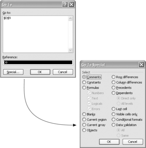
The selection methods described here are fairly common selection tasks that I use all the time. In some cases, even more control over selection is required. In this case, Excel has a feature that allows you to select cells based on some specific criterion (for example, cells that contain text or cells that contain numbers).

Press Ctrl-G or select Edit → Go To... from the main menu bar to open up the Go To dialog box. Then press the button labeled Special to open the Go To Special dialog box, as shown in Figure 1-9.

Figure 1-8. Group of selected cells

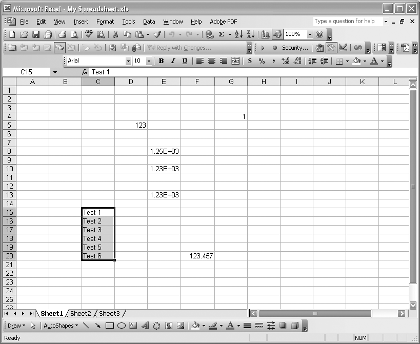
The Go To Special dialog box allows you to select or go to cells that correspond to the selected criterion. For the text selected in Figure 1-8, I selected the Constants criterion, which enabled the checkboxes below Formulas, at which point I made sure only Text was checked. You can do the same with numbers; for example, this is a convenient way to select all cells that contain only numbers, so that in a single shot you can change the number of decimal places shown for all numeric cells.

1.5. Entering Formulas

Problem

You’ve entered data and are ready to perform some calculations, but don’t know how.

Figure 1-9. Group of selected cells

Solution

You need to enter cell formulas in order to perform calculations on data contained in other cells. Entering a formula is simple enough: simply select a cell to hold the formula and then type the equals sign followed by your formula, which can refer to other cells that contain data. A formula to add two numbers contained in cells A1 and A2 would look like this: =A1+A2.

Discussion

All formulas start with an equals sign, as in the =A1+A2 example. You can enter a formula in the same way you enter text, as discussed in Recipe 1.2. You can either enter the formula directly in a cell (pressing Enter when done), or you can use the formula bar, as discussed earlier. The cell containing the formula will display the result of the formula and not the formula itself. To see the formula, just look at the formula bar when the cell is selected. Or press the F2 shortcut key to edit the formula directly in the cell, as shown in Figure 1-10.

Figure 1-10. Entering formulas

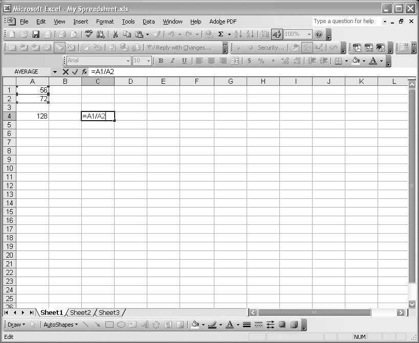
The cell in column C row 4 contains a formula to divide the number contained in column A row 1 by that in column A row 2. I pressed F2 to display the formula for editing directly in the cell.

Formulas may contain the usual mathematical operators such as +, -, /, and *, as well as any number of other built-in functions, as discussed in Recipe 1.10.

I should mention here that spreadsheets are a bit different from procedural programs with which you may be used to working. With a procedural program, you have to explicitly run it after writing the code (we’ll do this when we write custom macros and functions using Visual Basic for Applications in Chapter 2). However, once you write a formula in a spreadsheet cell, it executes and remains up-to-date automatically. Therefore, if you change the data in cells referred to by a formula, the results of the formula are updated immediately. Excel takes care of making sure your spreadsheet calculations are updated whenever you change anything.

Tip

Excel performs calculations on the stored values of cells (not the displayed values), using 15 digits of precision.

To really leverage formulas, you must understand cell references . In the formula =A1+A2, the data contained in the cells in rows 1 and 2 of column A are referenced as A1 and A2, respectively. In Excel such references are called A1-style references. The letter refers to the column; the number refers to the row number.

References to cells such as A1 are by default relative references . When a relative reference to a cell appears in a formula, that cell is referred to in terms of its relative position to the cell containing the formula. If you cut or copy the formula and then paste it someplace else, the cell references in the formula will automatically change so that they refer to cells in the same relative position to the formula as before. This is better explained by way of example.

In Figure 1-10, the cell A4 contains the formula =A1+A2, which uses relative references. If I copy and paste the formula from cell A4 to cell A5, then the new formula will be =A2+A3. I moved the formula one row down, so the relative cell references were also adjusted by one row. If I moved the formula to column B, then the cell references would have changed from A to B.

This behavior may seem a bit unusual at first, but the advantage of it is clear when you are setting up tables of data and formulas to manipulate the data. For example, say I had two columns of data, B and C, as shown in Figure 1-11.

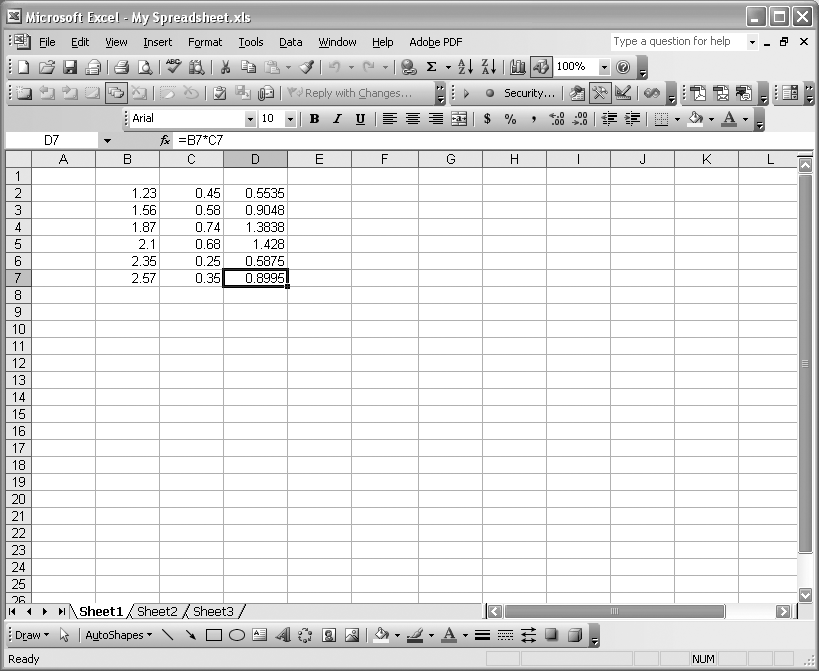
Figure 1-11. Relative cell references

Now in column D, I want to enter a formula to multiply each number in column B by the corresponding number (on the same row) in column C. To do this, I can enter the formula =B2*C2 in cell D2 to yield the product of numbers in cells B2 and C2. For all the remaining rows, I can simply copy and paste the formula in cell D2 into cells from D3 to D7, and Excel will automatically adjust the row numbers in the formulas. For example, after such copying and pasting, cell D7 contains the formula =B7*C7. This saves you the time of having to rewrite each formula directly. Relative cell references are also important when performing certain database filtering operations, as we’ll discuss later.

As useful as relative references are, they aren’t always want you want. Let’s say you have the data as shown in Figure 1-11, but instead of just taking the product of the two numbers in columns B and C, you want to also multiply this product by a single number contained in cell A1. Let’s say you want every product shown in column D to be multiplied by that same factor in cell A1. You might enter a formula in cell D2 like =B2*C2*A1. This works for the first result contained in cell D2, but if you copy and paste this formula into cells D3 through D7, the cell reference A1 will also be adjusted by 1 each time, resulting in the formula =(B7*C7)*A6 in cell D7. This isn’t want you want, since there are no values in cells A2 through A6. To force Excel to refer to a specific cell you need to use an absolute cell reference. This essentially fixes the cell reference to always refer to a specific cell no matter how the formula is moved or copied. The syntax for an absolute reference to cell A1 in our example looks like =(B2*C2)*$A$1.

The $ symbol in the cell reference indicates to Excel that you want to use absolute references. In this case we fixed both the column and the row in the example cell reference. If we wanted to fix just the column, we would write $A1. Likewise, we could fix just the row by writing A$1.

Tip

When entering a formula in a cell, you can select another cell from the spreadsheet to include that cell’s reference in the formula. You can also press F4 to cycle through the reference styles for the cell being referred to.

I use absolute references most often when performing calculations on datasets using formulas that refer to common scientific or engineering constants.

Tip

Formulas cannot refer to themselves. For example, if you put a formula in cell A3, it cannot contain a reference to cell A3. That’s called a circular reference, and Excel will give you a warning message if one occurs.

1.6. Exploring the R1C1 Cell Reference Style

Problem

You’ve seen the use of the A1 style of cell reference in Recipe 1.5 and are wondering if there are other ways to refer to cells.

Solution

Yes, there are other ways to refer cells, such as the R1C1 style.

Discussion

Besides using the A1 style of cell reference, you can also use the so-called R1C1 style of cell reference. This is not the default style, but in some cases it can be more intuitive or conducive to matrix operations and programming, as we’ll see later.

The R1C1 style uses numbers to identify both rows and columns in a spreadsheet. For example, R1C1 refers to the cell in row 1 column 1. To use the R1C1 style you must first activate it. To do so, go to the Tools → Options... menu to open the Options dialog box. Once it’s open, press the General tab (see Figure 1-12).

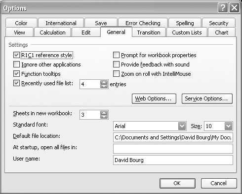
Figure 1-12. General tab in the Options dialog box

Check the box next to R1C1 reference style under the Settings heading to activate the R1C1 style. When you press OK and return to your spreadsheet, you’ll see that the column headings have changed from letters to numbers, as shown in Figure 1-13.

Figure 1-13. R1C1 reference style

Also notice that Excel automatically changed the formulas. For example, the formula in cell D7 (now R7C4) was =B7*C7; now it’s =RC[-2]*RC[-1], which is a relative reference in R1C1 style.

When using the R1C1 style, if you enter a cell reference like R3C5 (i.e., R followed by a number and C followed by another number), you are using absolute cell references. The equivalent in A1 style would be $E$3. Using brackets around the number following either R or C indicates relative cell references. For example, R[1]C[2] refers to the cell one row down and two rows to the right of the cell containing that reference. The cell two rows up and one row to the left would be referred to as R[-2]C[-1]. An R or C not followed by a number or a number in brackets refers to the same row or column as the cell containing the reference.

1.7. Referring to More Than a Single Cell

Problem

Sometimes you need to refer to a group of cells, not just a single cell. For example, some formulas discussed in Recipe 1.10 take more than a single cell as an argument. Thus you need to know the syntax for referring to more than one cell.

Solution

Use cell ranges .

Discussion

A cell range is simply a contiguous group of cells in rows or columns, or both. For example, the cell reference A1:A10 refers to the range of cells in column A from row 1 to row 10. The colon character (:) is used to indicate a range reference. The reference A1:B10 refers to the range of cells from column A row 1 to column B row 10. Technically speaking, the cell reference A1 is itself a range of only a single cell; thus, in a sense, all cell references can be thought of as ranges.

1.8. Understanding Operator Precedence

Problem

You want to learn the specific order in which Excel executes operations in formulas.

Solution

Excel performs operations in formulas from left to right following the leading equals sign. In doing so, Excel performs specific operations, if they are encountered in your formula, in the following order of precedence: negation, exponentiation, multiplication and division, and addition and subtraction.

Discussion

You can change operator precedence using parentheses. For example, if you enter the formula =A1+B2/C3 in a cell, Excel will perform the division first and then the addition. This may be what you want—that is, you want to add the result of B2 divided by C3 to A1. However, if you intend to divide the sum of A1 and B2 by C3, then you need to write =(A1+B2)/C3. The parentheses force Excel to perform the addition operation first, followed by the division.

You can also nest parentheses. For example you could write =((A1+B2)/C3)*C4, and so on. I find it is always good practice to use parentheses liberally to be sure your formula is executed as intended.

1.9. Using Exponents in Formulas

Problem

You need to write a formula that raises some number to some power but you don’t know the syntax for exponentiation in Excel.

Solution

Use the caret (^) operator.

Discussion

Raising a number to some power is a common calculation task. In Excel, the caret operator (^) is used for exponentiation. For example, to raise the number contained in cell A1 to the third power, you could enter the formula =A1^3. You can use whole number exponents as well as decimal numbers or even other operations. For example, the formulas =A1^0.25 and =A1^(1/4) both raise the value in cell A1 to the one-fourth power.

You need not hardcode exponents. You could use a number contained in another cell as an exponent; e.g., =A1^C5, or =A1^(C5+D10), or =(A1+A2)^(C5/E8), and so on.

1.10. Exploring Functions

Problem

The basic mathematical operators (+, -, /, *, and ^) are not enough to perform all the calculations you need.

Solution

Use Excel’s built-in functions, such as ABS( ), SQRT( ), and SIN( ), as needed.

Discussion

Throughout this book, I’m going to use all sorts of built-in functions in various calculations from data analysis to unit conversions to various engineering calculations. In this recipe I want to make you aware of the wide variety of built-in functions and how to access them in your spreadsheets.

Excel has many built-in functions, which can be organized in the following categories:

Database functions: Database functions include functions that allow you to get information from database entries and perform some statistical analyses of data contained in databases.
Date and time functions: Date and time functions include functions that allow you work with and perform calculations using dates and times. For example, you may want to calculate the number of working days between two dates, in which case you can use the NETWORKDAYS function. There are many others, including functions to get the current date and time.
Engineering functions: Engineering functions include functions that allow you to work with complex numbers, convert between number systems, and convert between systems of measurement. There are also many other specialized functions for working with Bessel and Delta functions, among others.
Financial functions: Financial functions include many functions that help you analyze things like accrued interest, depreciation, annuities, and investments, among many others.
Logical functions: Logical functions include a small set of useful logical functions . For example, the IF function allows you to evaluate a logical expression and return one value if the expression is true and another value if it is false. There are other functions including AND, OR, and NOT, among others, that help you construct logical expressions.
Lookup functions: Lookup functions are useful for looking up data in tables, matching values, returning rows or columns for cell references, and other tasks.
Math functions: Math functions help you perform calculations, and include operations such as taking the absolute value of a number, finding square roots, working with logarithms and exponential functions, summing values of data contained in rows or columns, and working with trigonometric functions. This is perhaps the most used set of functions for the sorts of calculations discussed in this book.
Statistical Functions: Statistical functions are useful for calculating averages, standard deviations, variances, among many other calculations. There is also a set of functions useful for working with probability and distributions, including binomial, Weibull, and normal distributions, among others.
Text and data functions: Text and data functions include a set of functions for manipulating text and converting numeric data to text. For example, there are functions to compare text strings, search for a substring within a larger text string, convert a string to all upper- or lowercase, and replace characters within a string.

There are a few other categories of built-in functions that I didn’t summarize here. These functions are rather specialized and are useful for working with external programs and databases and collecting information from the host operating system, among other tasks.

The recipes throughout the remainder of this book will use many built-in functions, most notably, but not limited to, the math, statistical, engineering, and logical functions. I’m not going to list all of the available functions here, since they are already documented fairly well within Excel itself and there are also many books that serve as complete Excel function references. I do want to show you how to access these built-in functions now so you can be familiar with the process when you read the more specific recipes to follow in later chapters of this book.

The easiest way to use a function in a formula is to simply type the function. For example, to sum the values contained in a column consisting of the cell range C1:C10, you can write a formula using the SUM function like this: =SUM(C1:C10). In this case, SUM is the function and the cell range is the argument of the function.

When typing such a formula in a cell, as soon as you type the opening parenthesis after the function name, Excel will display a small, helpful information box below your formula, showing what arguments are expected (assuming you’ve typed a valid built-in function and spelled it correctly). At this point, you can type the arguments directly or, if the argument calls for a cell range, you can actually point and click to select the cell range, and Excel will automatically complete the cell reference argument for you. This reduces working with cell references in formulas to a point-and-click operation rather than typing everything out manually.

When typing a function, if you’d like more help on the function aside from the argument list that’s automatically displayed, you can press the f _x icon (called the Insert Function button ) in the formula bar to display the Function Arguments dialog box (see Figure 1-14).

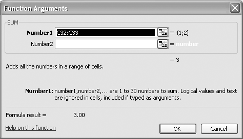
Figure 1-14. Function Arguments dialog box

The Function Arguments dialog box displays controls and notes to help you construct the arguments for the function. There’s also a link to more help on the specific function, as shown in the lower-left corner of the dialog box in Figure 1-14.

Of course, the method of using functions discussed so far requires that you at least know the function name that you’d like to use. If you don’t know or can’t remember the name, you can either look it up in Excel Help or you can use the formula bar and the Insert Function dialog box to help you find appropriate functions.

To use the Insert Function dialog, select the formula bar to begin writing a formula and then press the f _x icon when you need to look up a function. This will bring up the Insert Function dialog box (see Figure 1-15).

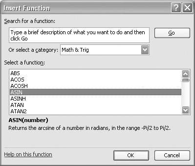
Figure 1-15. Insert Function dialog box

With the Insert Function dialog box open, you may type a short description of what you’re looking for in the “Search for a function” field. Or you can select a category from the drop-down list to view a list of functions within that category. From there you can select the specific function you need and press OK. When you press OK, the Function Argument dialog box will open to assist you with supplying function arguments. When you press OK in the Function Argument dialog box, you’ll see your selected function, including arguments, appear in the formula bar; at this point, you can continue writing your formula.

Tip

You can nest functions. For example, you can use a formula like =SQRT(ABS(C5)) to return the square root of the absolute value of the value contained in cell C5.

1.11. Formatting Your Spreadsheets

Problem

You’ve got data and some calculations, but the spreadsheet looks unpresentable.

Solution

Format your spreadsheet to make it more presentable and better organized.

Discussion

In Recipe 1.3, I discussed how to format cells to specify the type of data (e.g., text, numbers, currency, etc.). In this recipe, I’ll show you a few other formatting techniques. Take a look at the spreadsheet in Figure 1-16.

This simple spreadsheet merely calculates values for a function of the form y = x ⁿ, where n is the exponent shown on the spreadsheet. It also calculates the cumulative area under the curve from 0 to x. The results are plotted on a chart adjacent to the calculation table. Chapter 4 covers charting in detail, so I won’t discuss the chart here. Instead I want to focus on the calculation table.

I could have simply filled in a column of x values, entered formulas for the y and area values, and left it at that. However, that would look messy. More than likely you’ll want to include your calculations in reports or share them with others, so making your spreadsheets presentable is a good idea. Formatting also serves as a form of documentation so that you can come back to a spreadsheet weeks or years later and quickly see what you did. There’s (almost) nothing worse than opening an old spreadsheet and seeing just a grid of scattered numbers.

Figure 1-16. Formatted spreadsheet

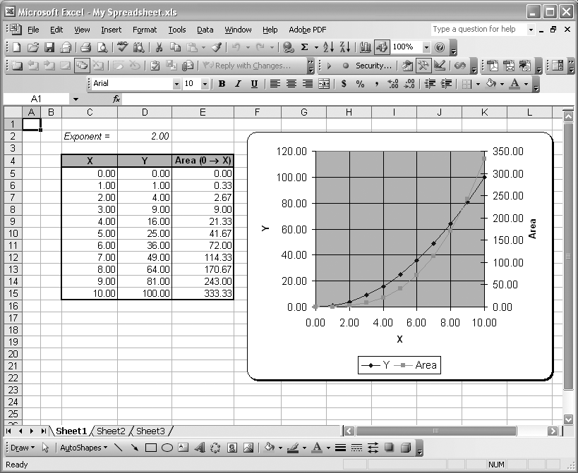
There are many ways to format your spreadsheet. In this example, I added a text label, in italics, in the cell C2 to indicate the purpose of the value in cell D2. I also added some borders around the table of calculations and delineated the column headings with a filled background and bold text. I also centered the column labels above the data instead of using the default left justification for text. If you’re a keen observer, you may have noticed that I also changed the column width of several columns—I reduced the width of columns A and B so they wouldn’t take up too much space and I increased the width of column E to accommodate the area column label. These are some of the most common formatting tasks I make on virtually every spreadsheet I write. They are simple and effective.

You can access Excel’s formatting functions via the Format menu . There you’ll find options for formatting cells, whole rows or columns, and even the entire spreadsheet. I personally use the cell formatting options the most. You’ve already seen how to access the Format Cells dialog box in Recipe 1.3, and as shown in Figure 1-6. You can use the main menu bar or the shortcut key combination, Ctrl-1, to open the Format Cells dialog box.

The Number tab displays the data type formatting options discussed earlier. The other tabs give you control of other cell aspects:

Alignment: Set the position, orientation, and justification of text within a cell. You can also specify whether long text should wrap around, creating multiple lines of text in a single cell.
Font: Specify the font type, style, and size of text to appear in a cell. For example, you could specify Arial font type with a bold style and a size of 10 points.
Border: Add borders to any edge of a cell. You can select from a variety of line styles, including solid, dashed, and dotted, among others, and even set the line thickness.
Patterns: Set the background color or pattern for a cell.
Protection: Specify whether a cell is protected (meaning it can’t be changed without a password) and whether a cell is hidden.

While the Format Cells dialog box presents you with many cell formatting options, I prefer to use the toolbars for quick formatting tasks. If you look closely at Figure 1-16, you’ll see the formatting toolbar visible just above the formula bar. This toolbar contains buttons to change a cell’s font, justification, data type, number of decimal places, indention, borders, fill patterns, text color, and more. You can customize this toolbar as discussed in Recipe 1.1.

There may be times when you want to clear all the formats applied to a cell. To do so, select the cell whose formats you want to clear and then select Edit → Clear → Formats from the main menu bar.

1.12. Defining Custom Format Styles

Problem

You find yourself applying the same formats repeatedly to different cells and would like to save time when doing so.

Solution

Define your own custom style and apply it to cells, taking care of many format settings all in one step.

Discussion

Select Format → Style from the main menu bar to open the Style dialog box as shown in Figure 1-17.

Figure 1-17. Style dialog box

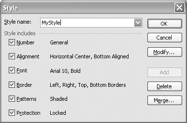
The drop-down combo box next to the “Style name” label contains a list of predefined styles that you can apply to cells. Some of these are familiar, including the normal cell style along with currency and percent styles. You can add your own style to this list. Click the combo box, type in a unique name for your new style, and then press the Add button. Now you can check off the format options you want to include in your style and modify the format settings by pressing the Modify button. Pressing the Modify button opens the Format Cells dialog box (see Figure 1-6 in Recipe 1.3). You can make any format selection you desire and close this dialog box when done. The settings you specified will be applied to your custom style.

Once your style is defined, you have a few options for actually using it to format cells. One way to apply your custom style is to select the desired cell (or cells) and then select Format → Style... from the main menu bar to open the Style dialog box again. There you can select your desired style and press OK to close the dialog box. Your style will then be applied to the selected cell (or cells).

A faster approach involves adding a style drop-down list component to one of the toolbars on the main window so that you can simply select cells and then select a style to apply from the toolbar.

To add a style drop-down list to a toolbar, select View → Toolbar → Customize... from the main menu bar to open the Customize dialog box. Select the Commands tab (shown in Figure 1-18).

Figure 1-18. Customize dialog box

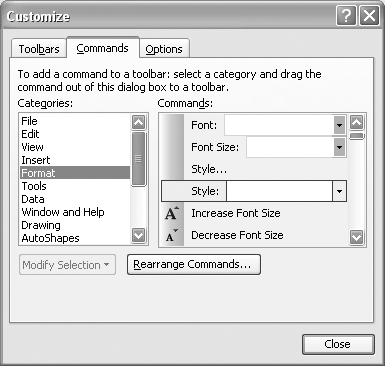
Now select Format from the Categories list to show the format commands. From the Commands list look for the Style drop-down listbox shown in Figure 1-18. Don’t confuse it with the Style... dialog box command. Click and drag the Style listbox control from the Commands list over to any toolbar, preferably the format toolbar, on Excel’s main window. After you close the Customize dialog box, that listbox will be available to you on the toolbar.

To use the Style listbox, select the cells to which you want to apply a style and then select the desired style from the Style listbox that you added to the toolbar.

1.13. Leveraging Copy, Cut, Paste, and Paste Special

Problem

You’d like to take advantage of standard Windows copy-and-paste functionality but aren’t familiar with the caveats for doing so within Excel.

Solution

Read the following discussion.

Discussion

Under Excel’s Edit menu , you’ll find the usual Cut, Copy, and Paste menu items. For the most part, these work just as they do in any other Windows program. To move the contents of a cell from one place to another, use the Cut and Paste operations. To copy a cell into other cells, use the Copy and Paste operations. There are a few things to be aware of when performing these operations in Excel:

When you cut or copy and then paste, all of the cell’s attributes are copied, along with the data or formula that it contains. This means things like font, alignment, borders, and patterns will be copied as well.
When you cut and paste data to a new location, any formulas referring to its original cell location are automatically updated to refer to its new location. Copying a cell to another location has no effect on formulas that refer to the original cell.
When you copy a cell containing a formula, relative cell references in the formula will be adjusted by the relative distance of the pasted cell from the copied cell.
When you cut a formula and paste it to a new location, the formula will remain unchanged; i.e., it should still refer to the same cells and give the same results as before the cut-and-paste operation.

Sometimes you may want to cut or copy and then paste all of the format settings and data from one cell to another. In cases when you don’t, you can use the Paste Special option, which is also under the Edit menu. When you select the Paste Special option, a dialog box like that shown in Figure 1-19 appears.

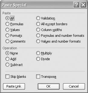
Figure 1-19. Paste Special dialog box

Here you can select exactly what it is you want to copy and paste. For example, if you want to copy and paste only cell format settings, you can select the Formats option. Similarly, if you want to copy and paste just a formula and not the cell’s formatting, then you can select the Formulas option, and so on.

The Operation options allow you to specify some basic mathematical operations to perform on the data being copied and the contents of the destination cell. For example, say you copy a number from one cell and Paste Special it to a cell that already contains another number. If you select the Add option, the sum of the two cell values will be entered in the destination cell.

The “Skip blanks” option excludes empty cells from the selected range of cells being copied. The Transpose option is similar to a matrix transpose operation. For example, if you copy a column of numbers and paste it with the Transpose option, it will be converted to a row of numbers.

Here are some handy keyboard shortcuts for the basic cut-and-paste operations:

Cut: Ctrl-X
Copy: Ctrl-C
Paste: Ctrl-V

There is no shortcut for the Paste Special operation; however, you can right-click anywhere in your spreadsheet to bring up a pop-up menu containing the Paste Special option. I find this quicker than accessing the main menu bar.

Tip

Cut, Copy, Paste, and other options (e.g., Format Cells) are also shown on the right-click pop-up menu.

1.14. Using Cell Names (Like Programming Variables)

Problem

You frequently use a particular cell in formulas and are tired of typing the reference. You’d like a more descriptive syntax, similar to that used for variable or constant names in traditional programming languages.

Solution

Use cell names .

Discussion

Select the cell or cell range for which you want to define a name. Next, select Insert → Name → Define... from the main menu bar to open the Define Name dialog box (see in Figure 1-20).

Figure 1-20. Define Name dialog box

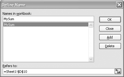
Enter a name for the selected cell range in the edit field under “Names in workbook.” Make sure the “Refers to” field does indeed refer to the cell range you’d like to name. If you had the range selected when you opened this dialog box, then the cell range should already be correct. If you didn’t have it selected, press the icon in the lower-right corner; this will allow you to select the proper range without leaving the Define Name dialog box. Once your name is entered and the cell reference is correct, press the Add button. You’ll now be able to use that name to refer to the associated cell range in any formulas in your workbook.

Notice that the cell reference in the “Refers to” field in Figure 1-20 includes the sheet name, Sheet1, followed by the exclamation mark (!), which precedes the absolute A1-style cell reference. This format, using the sheet name followed by !, makes the reference refer to the specified cell on that specific sheet. Thus, you can use the name in a formula on any other sheet and it will still point to the cell on Sheet1.

Tip

I find names quite useful. Typically, if I’m performing calculations that require the use of empirical constants or commonly used data, I’ll set up a specific sheet in my workbook that contains only constants and commonly used data (or formulas). Then I name these so I can refer to them throughout the workbook. I find descriptive names more intuitive and easier to remember than cryptic cell references that span sheets in a workbook.

1.15. Validating Data

Problem

You want to make sure users of your spreadsheet don’t enter inappropriate data.

Solution

Use Excel’s Data Validation feature.

Discussion

Excel allows you to specify what constitutes valid data for any given cell. For example, say you had a spreadsheet that performed some calculations given a value that was input in a particular cell by a user other than yourself. Let’s say you want to restrict the range of values the user can enter in the input cell, in order to minimize the possibility of misuse. Such a situation could arise if, say, you write a spreadsheet that allows you to interpolate data based on a regression equation. In such a case, you would want to restrict the independent value input by the user to within the allowable bounds of the regression analysis. Basically, you don’t want the user to attempt to extrapolate beyond the data range used in the regression analysis, as such extrapolations can sometimes yield dangerously inaccurate results.

To specify validation for a cell, select the cell you want to set validation for and then open the Data Validation dialog box by selecting Data → Validation... from the main menu bar. Figure 1-21 shows the Data Validation dialog box.

Figure 1-21. Data Validation dialog box

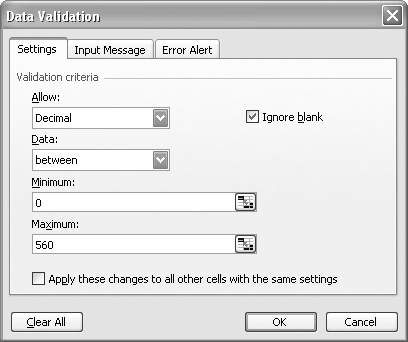
The Allow drop-down listbox allows you to select the type of data to allow (for example, a decimal number, a whole number, a date, or text). Once you select the Allow type, the other controls will present additional qualifiers. In the example shown in Figure 1-21, I set 0 to 560 as the valid data range. You can also specify ranges greater than some value, less than some value, and so on. Once you press OK, these changes take effect. If the user attempts to enter data that does not fit the valid data criteria, a message box will appear indicating bad data entry.

Tip

You can specify exactly what you want the error message to display by entering your message under the Error Alert tab of the Data Validation dialog box. Further, clicking the Input Message tab allows you to specify an information message to be displayed to the user whenever a cell using data validation is selected. This is useful for giving your users a clue as to what constitutes valid data for any particular cell.

1.16. Taking Advantage of Macros

Problem

You find yourself repeating the same actions over and over and would like to automate that process.

Solution

Use Excel’s macro-recording feature to record your actions, which can then be executed again using a keyboard shortcut.

Discussion

Let’s say you find yourself repeatedly applying the same format settings to cells; for example, you select a cell, set the font style to bold, set justification to center, and apply a pattern and a border. You could define a custom style reflecting these format settings and use the style as discussed in Recipe 1.12, or you could record a macro to automate the process of setting these formats.

Although I’m using formats as an example, you should be aware that the macro-recording feature lets you record any sequence of actions taken in Excel, thus allowing you to automate almost anything. In Chapter 2, I discuss macros and other programming tasks in much greater detail in the context of using Visual Basic for Applications. That said, you can record simple macros to automate common tasks as discussed here, without using Visual Basic.

Take these steps to record a macro:

Select Tools → Macro → Record New Macro... from the main menu bar to open the Record Macro Dialog box.
In the Macro Dialog box, enter a descriptive name for your new macro in the Macro Name field. Also enter a shortcut letter for the shortcut key combination (Ctrl plus the letter you specify), which will be used to execute the macro on demand. In the Store Macro In field, select where you want the macro stored. The default is This Workbook, which stores the macro in the current workbook. However, if you want to be able to use the macro in any workbook, you should select Personal Macro Workbook. Press OK when you’re done; this will return you to the spreadsheet in macro-recording mode.
Execute the actions you want recorded.
When you’ve finished your actions, select Tools → Macro → Stop Recording from the main menu bar.
Use the shortcut key you specified in the Macro Dialog box to execute your macro.

Let’s say you recorded a series of cell-formatting actions in a macro. Then, anytime you select a cell and press the shortcut key for that macro, the macro will run and you’ll see that formatting applied to the cell.

If you want the macro to execute relative to the position of the active cell when you start recording, make sure the Relative Reference button is selected on the Record Macro toolbar that appears when you start recording a macro. The Relative Reference button is shown in Figure 1-22.

Figure 1-22. Record Macro toolbar

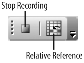
You may also press the Stop Recording button to stop recording a macro (instead of using the Stop Recording menu item as mentioned earlier).

To manage macros, you can access the Macro dialog box via the Tools → Macro → Macros... menu or the Alt-F8 shortcut. The Macro dialog box allows you to run selected macros, delete macros, or redefine their shortcut keys.

1.17. Adding Comments and Equation Notes

Problem

You’d like to add comments to your spreadsheet, just as you’d comment your code in a traditional programming language.

Solution

Aside from simply inserting text in cells adjacent to cells containing data or formulas, you can use comments or equation objects to document your spreadsheets.

Discussion

Figure 1-23 shows a sample spreadsheet that includes a comment and an equation object documenting parts of the spreadsheet.

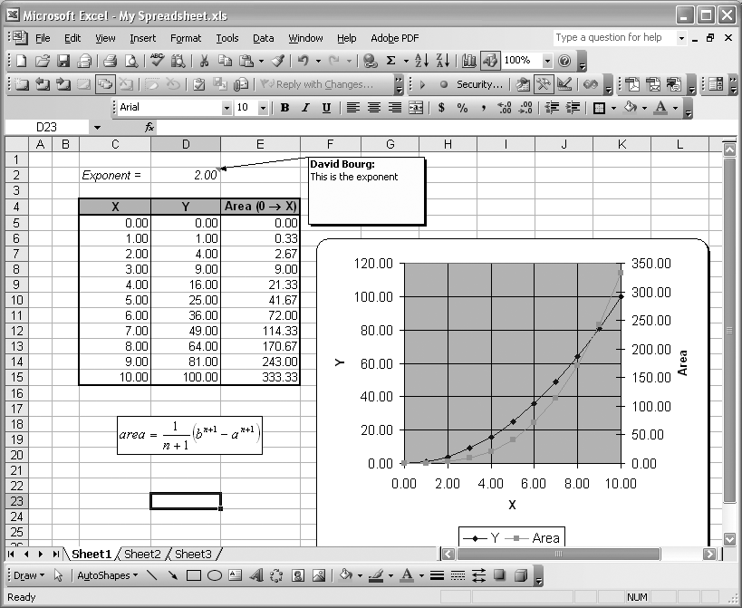
Figure 1-23. Spreadsheet with comment and equation

The comment is the rectangle containing the text “David Bourg: This is the exponent,” with an arrow pointing to cell D2. The equation object is the rectangle containing the mathematical expression for the area calculation. Both comments and equations are useful devices for documenting your spreadsheets. I often use comments to leave myself notes or reminders or to-do lists within my spreadsheets. I use equations to document formulas used in my spreadsheets that will be used by others or included in reports or other presentations. Equations in standard mathematical form are much clearer and far easier to comprehend than cell formulas containing a bunch of cell references and operators all strung together.

To add a comment, first select the cell to which you want the comment attached, then select Insert → Comment from the main menu bar. A comment box will appear (with input focus, so you can immediately begin typing your comment). When you’re done typing, use the mouse to select where on the spreadsheet you want the comment box to be placed. To edit an existing comment, select the cell containing the comment and select Insert → Edit Comment from the main menu bar. This will give input focus to the comment, allowing you to edit its message. To delete a comment, select the cell containing the comment and right-click to reveal a pop-up menu where you can select Delete Comment to actually delete the comment.

Tip

You can also use the Reviewing toolbar (by selecting View → Toolbars → Reviewing) to access comment features such as adding, editing, deleting, or temporarily hiding comments.

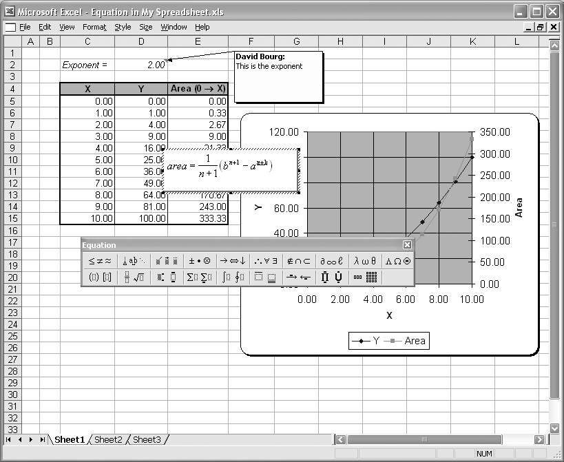
To add an equation, you need to use the Microsoft Equation Editor to insert an equation object into your spreadsheet. Select Insert → Object... to show the Object Dialog box. From the list of Object Types in this dialog box, choose Microsoft Equation 3.0. When you press OK, the dialog will close, returning you to the spreadsheet in equation-editing mode (see Figure 1-24).

The equation rectangle will appear, allowing you to enter an equation using the equation toolbar shown in Figure 1-24. You can type text in the equation using the keyboard. To insert mathematical symbols, select them from the equation toolbar. Use the arrow keys on the keyboard to navigate an equation while editing. The Equation Editor is a bit cumbersome at first; I suggest you try it and practice until you get the hang of it. When you’re done entering an equation, simply click anywhere in your spreadsheet to close the Equation Editor. You can click and drag the resulting equation to place it anywhere in your spreadsheet. To edit an existing equation, select it and then right-click on it to reveal a pop-up menu. Select Equation Object → Edit from this pop-up menu to edit the equation. To delete an equation, simply select it and press the Delete key on your keyboard.

Figure 1-24. Editing an equation

Tip

The Equation Editor discussed here is the same one that’s accessible from Microsoft Word . You can insert equations in your Word documents in the same way that you add equations to a spreadsheet, and you don’t have to have Excel open in order to do so. This is useful for preparing technical reports in Word.

1.18. Getting Help

Problem

You’re off to a great start and would like to know where you can go to find help within Excel .

Solution

You can access Excel’s online help system by selecting Help → Microsoft Excel Help from the main menu bar. Or you can use the shortcut Ctrl-F1 to access the Help task pane, enabling you to select the Excel Help page, where you can click the “Table of Contents” link or enter a search phrase to search for help topics.

Get Excel Scientific and Engineering Cookbook now with the O’Reilly learning platform.

O’Reilly members experience books, live events, courses curated by job role, and more from O’Reilly and nearly 200 top publishers.

Start your free trial

Chapter 1. Using Excel

Introduction

1.1. Navigating the Interface

Problem

Solution

Discussion

Tip

Main menu bar

Task pane

Tip

Toolbars

Tip

See Also

1.2. Entering Data

Problem

Solution

Discussion

1.3. Setting Cell Data Types

Problem

Solution

Discussion

See Also

1.4. Selecting More Than a Single Cell

Problem

Solution

Discussion

See Also

1.5. Entering Formulas

Problem

Solution

Discussion

Tip

Tip

Tip

See Also

1.6. Exploring the R1C1 Cell Reference Style

Problem

Solution

Discussion

See Also

1.7. Referring to More Than a Single Cell

Problem

Solution

Discussion

See Also

1.8. Understanding Operator Precedence

Problem

Solution

Discussion

1.9. Using Exponents in Formulas

Problem

Solution

Discussion

See Also

1.10. Exploring Functions

Problem

Solution

Discussion

Tip

See Also

1.11. Formatting Your Spreadsheets

Problem

Solution

Discussion

See Also

1.12. Defining Custom Format Styles

Problem

Solution

Discussion

1.13. Leveraging Copy, Cut, Paste, and Paste Special

Problem

Solution

Discussion

Tip

1.14. Using Cell Names (Like Programming Variables)

Problem

Solution

Discussion

Tip

1.15. Validating Data