Feedback Control for Computer Systems

Chapter 1. Why Feedback? An Invitation

Workflow, order processing, ad delivery, supply chain management—enterprise systems are often built to maintain the flow of certain items through various processing steps. For instance, at a well-known online retailer, one of our systems was responsible for managing the flow of packages through the facilities. Our primary control mechanism was the number of pending orders we would release to the warehouses at any one time. Over time, these orders would turn into shipments and be ready to be loaded onto trucks. The big problem was to throttle the flow of pending orders just right so that the warehouses were never idle, but without overflowing them (quite literally) either.

Later I encountered exactly the same problem, but in an entirely different context, at a large publisher of Internet display ads. In this case, the flow consisted of ad impressions.^[1] Again, the primary “knob” that we could adjust was the number of ads released to the web servers, but the constraint was a different one. Overflowing the servers was not a concern, but it was essential to achieve an even delivery of ads from various campaigns over the course of the month. Because the intensity of web traffic changes from hour to hour and from day to day, we were constantly struggling to accomplish this goal.

As these two examples demonstrate, maintaining an even flow of items or work units, while neither overwhelming nor starving downstream processing steps, is a common objective when building enterprise systems. However, the changes and uncertainties that are present in all real-world processes frequently make it difficult, if not impossible, to achieve this goal. Conveyors run slower than expected and web traffic suddenly spikes, disrupting all carefully made plans. To succeed, we therefore require systems that can detect changes in the environment and respond to them.

In this book, we will study a particular strategy that has proven its effectiveness many times in all forms of engineering, but that has rarely been exploited in software development: feedback control. The essential ingredient is that we base the operations of our system specifically on the system’s output, rather than on other, more general environmental factors. (For example, instead of monitoring the ups and downs of web traffic directly, we will base our delivery plan only on the actual rate at which ads are being served.) By taking the actual output into account (that’s what “feedback” means), we establish a firm and reliable control over the system’s behavior. At the same time, feedback introduces complexity and the risk of instability, which occurs when inappropriate control actions reinforce each other, and much of our attention will be devoted to techniques that prevent this problem. Once properly implemented, however, feedback control leads to systems that exhibit reliable behavior, even when subject to uncertainty and change.

A Hands-On Example

As we have seen, flow control is a common objective in enterprise systems. Unfortunately, things often seem rigged to make this objective difficult to attain. Here is a typical scenario (see Figure 1-1).

1. We are in charge of a system that releases items to a downstream processing step.

2. The downstream system maintains a buffer of items.

3. At each time step, the downstream system completes work on some number of items from its buffer. Completed items are removed from the buffer (and presumably kicked down to the next processing step).

4. We cannot put items directly into the downstream buffer. Instead, we can only release items into a “ready pool,” from which they will eventually transfer into the downstream buffer.

5. Once we have placed items into the ready pool, we can no longer influence their fate: they will move into the downstream buffer owing to factors beyond our control.

6. The number of items that are completed by the downstream system (step 3) or that move from the ready pool to the downstream buffer (step 5) fluctuates randomly.

7. At each time step, we need to decide how many items to release into the ready pool in order to keep the downstream buffer filled without overflowing it. In fact, the owners of the downstream system would like us to keep the number of items in their buffer constant at all times.

Figure 1-1. Block diagram of a workflow system. Items are being released into the “ready pool,” from which they are transferred to the downstream buffer.

It is somewhat natural at this point to say: this is unfair! We are supposed to control a quantity (the number of units in the downstream buffer) that we can’t even manipulate directly. How are we supposed to do that—in particular, given that the downstream people can’t even keep constant the number of items they complete at each time step? Unfortunately, life isn’t always fair.

Hoping for the Best

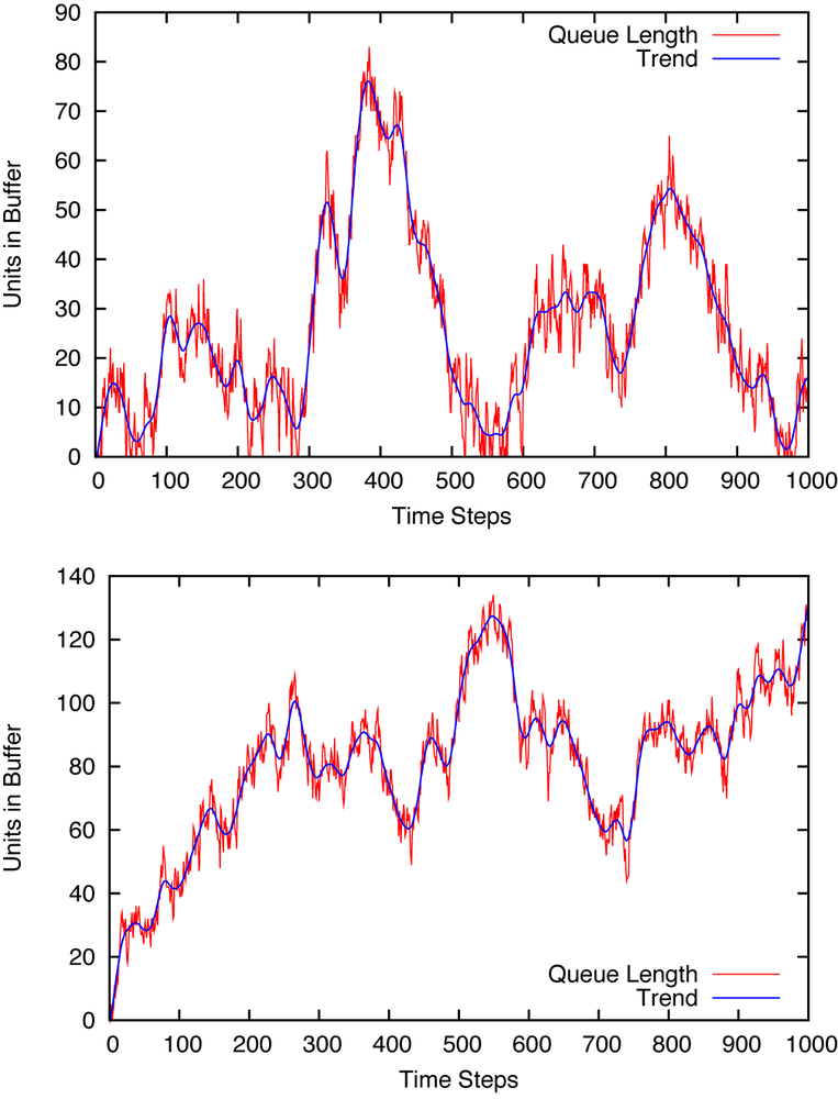
What are we to do? One way of approaching this problem is to realize that, in the steady state, the number of units flowing into the buffer must equal the number of units flowing out. We can therefore measure the average number of units leaving the buffer at each time step and then make sure we release the same number of units into the ready pool. In the long run, things should just work out. Right?

Figure 1-2 (top) shows what happens when we do this. The number of units in the buffer (the queue length) fluctuates wildly—sometimes exceeding 100 units and other times dropping down to zero. If the space in the buffer is limited (which may well be the case if we are dealing with a physical processing plant), then we may frequently be overflowing the buffer. Even so, we cannot even always keep the downstream guys busy, since at times we can’t prevent the buffer from running empty. But things may turn out even worse. Recall that we had to measure the rate at which the downstream system is completing orders. In Figure 1-2 (bottom) we see what happens to the buffer length if we underestimate the outflow rate by as little as 2 percent: We keep pushing more items downstream than can be processed, and it doesn’t take long before the queue length “explodes.” If you get paged every time this happens, finding a better solution becomes a priority.

Figure 1-2. Number of units in the buffer as a function of time, where the consumption rate is equal to the inflow (top) or slightly smaller than the inflow (bottom).

Figure 1-3. Number of units in the buffer, after the introduction of a controller that bases the inflow on the buffer’s current fill level, for two different values of the controller gain k.

Establishing Control

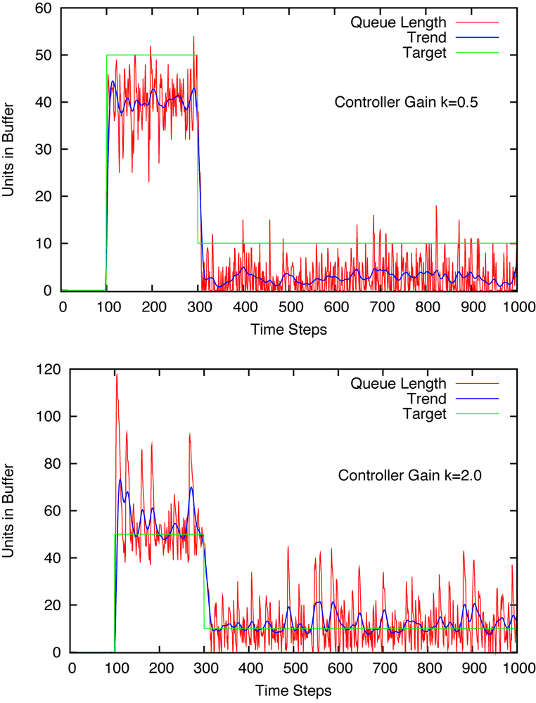
Clearly, we need to come up with a better idea. The first step is to stop relying on the “average” outflow rate (which, by the way, may itself be changing as time goes on). Instead, we will monitor the actual length of the queue from moment to moment. In fact, we will ask the downstream team to give us a target: a specific queue length that they want us to maintain. We will then compare the actual queue length to the target. Only if the actual length is below the desired value will we release additional units into the ready pool. Moreover—and this is important—we will let the number of units released depend on the magnitude of the deviation: If the actual queue length is only slightly below the target, then we will release fewer units than if the queue length is way off the mark. Specifically, we will use the following formula to calculate the number of units to release into the ready pool:

released units = k · (target – actual)

where k is a numerical constant. How large should k be? Aye, there’s the rub. We don’t know yet. Why don’t we take k = 0.5 for starters—that seems like a safe value.

Figure 1-3 (top) shows the actual queue length together with the desired target value. (Notice that the target value changes twice during the period shown.)

Two things are immediately clear:

• We are doing a much better job keeping the queue length approximately constant. In fact, we are even able to follow the two changes in the target value without too much trouble.

• Nevertheless, we don’t really manage to match the target value exactly—the actual queue length falls short of the desired value. This shortfall is especially pronounced for later times, when the target itself is small: instead of the desired 10, we only manage to keep the queue length at around 3. That’s quite a bit off!

Can we improve on our ability to track the target if we increase k (the “controller gain”)? Figure 1-3 (bottom) shows what happens if we set k = 2.0. Now the actual queue length does match the target in the long run, but the queue length is fluctuating a great deal. In particular, when the system is first switched on we overshoot by more than a factor of 2. That’s probably not acceptable.

In short, we are clearly on a good path. After all, the behavior shown in Figure 1-3 is incomparably better than what we started with (Figure 1-2). Yet we are probably still not ready for prime time.

Adding It Up

If we reflect on the way our control strategy works, we can see where it falls short: we based the corrective action (that is, the number of units to be released into the ready pool) on the magnitude of the deviation from the target value. The problem with this procedure is that, if the deviation is small, then the corrective action is also small. For instance, if we set k = 0.5, choose 50 as a target, and the current length of the queue is 40, the corrective action is 0.5 · (50 – 40) = 5. This happens to be approximately the number of units that are removed from the buffer by the downstream process, so we are never able to bring the queue length up to the desired value. We can overcome this problem by increasing the controller gain, but with the result that then we will occasionally overshoot by an unacceptable amount.

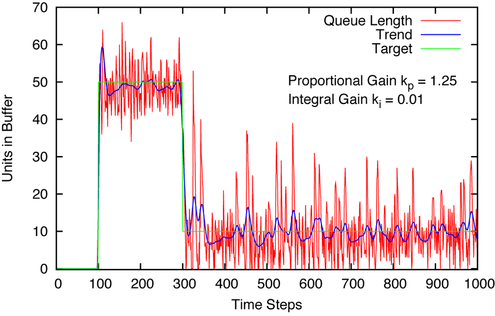
The remedy is to magnify the effect of persistent small deviations by adding them up! After a few time steps, their influence will have grown sufficiently to make itself felt. However, if the deviations are reliably zero, then adding them up does not make a difference. Hence we modify our control strategy as follows. We still calculate the tracking error as (target – actual) at each time step, but we also keep a running sum of all tracking errors up to this point. We then calculate the number of units to be released as the combination of the two contributions:

released units = k_p · error + k_i · cumulative error

Now we have two numerical factors to worry about: one (k_p) for the term that is proportional to the error, and one (k_i) for the term that is proportional to the cumulative sum (or: the “integral”) of the error. After some trial and error, we can obtain a result that’s quite adequate (see Figure 1-4).

Figure 1-4. The number of units in the buffer when using a controller that contains both a proportional and an integral term.

Summary

The method we have utilized in this chapter is called feedback. The goal of using feedback control is to make a system’s output track a reference signal as closely as possible. This is achieved by continuously comparing the output signal to the reference and applying a corrective action to reduce the tracking error. Moreover, the magnitude of the corrective action depends on the magnitude of the tracking error.

Feedback is a fairly robust control strategy—using feedback, one can successfully track a reference signal even in the face of uncertainty. The reason for the uncertainty does not matter: it may be due to random effects (“noise,” as in our queueing example); it may be due to our lack of knowledge about the inner workings of a complicated, “black-box” system that we need to control. In contrast, feedforward control—whereby we attempt to work out all decisions ahead of time—requires precise knowledge of all applicable laws yet still remains vulnerable to the detrimental effects of inaccuracy and uncertainty.

The behavior of systems involving feedback loops can be complicated and hard to predict intuitively. In particular, we run the danger of introducing instability: a corrective action leads to overshoot, which in turn is corrected by an even greater overshoot in the opposite direction, in a rapidly escalating pattern. Even if such catastrophic blow-ups can be avoided, it is often the case that feedback-controlled systems exhibit undesirable oscillatory behavior (control oscillations).

The desire to avoid instability in feedback loops has led to the development of a deep and impressive theory describing such systems but also to a set of heuristics and simple “rules of thumb” for practical applications. Part II of this book provides an overview of some of these heuristic tuning and design methods, and Part IV offers a brief introduction to the central theoretical methods and results.

Let’s close this first look with some general observations about feedback control and the types of situations where it is most applicable.

• Feedback control applies an automatic correction to deviations from a reference signal. This allows for tighter control but is accompanied by a tendency toward oscillatory or even unstable behavior.

• Feedback is about tracking a given reference signal. Without a reference signal, there can be no feedback control.

• It follows that feedback is about control, not about optimization. A task such as “make the flow through the system as large as possible” can not be solved by feedback alone—instead, such a task requires an optimization strategy. However, feedback may prove extremely useful if not necessary when you are seeking to implement or execute such a strategy.

• Frequent, small changes are better suited to stabilizing a system than rare, large changes. If we are unable to observe the system constantly and apply corrective actions frequently, then feedback won’t work.

• The choice of reference signal will often be determined by an existing optimization strategy. In contrast, what is considered to be a system’s “input” and “output” is arbitrary and depends on the objectives and any existing constraints. In our example, we tried to maintain a constant queue length in the buffer. Alternatively, we could have tried, for example, to maintain a certain throughput through the entire system. Identifying the most suitable input/output variables to accomplish the desired task most easily can be a real challenge, especially when applying feedback control to a “nonstandard” situation.

Code to Play With

The graphs in Figure 1-2 through Figure 1-4 were produced using a simulation of the buffer system described. The simulation is simple, so it is easy to add your own extensions and variations. Play around with this system a little: make some changes and see how it affects the outcomes. It is extremely helpful to develop some experience with (and intuition for) the effects that feedback control can have!

We begin with the class for the entire buffer system, including what we have called the “ready pool.”

class Buffer:
    def __init__( self, max_wip, max_flow ):
        self.queued = 0
        self.wip = 0       # work-in-progress ("ready pool")

        self.max_wip = max_wip
        self.max_flow = max_flow # avg outflow is max_flow/2

    def work( self, u ):
        # Add to ready pool
        u = max( 0, int(round(u)) )
        u = min( u, self.max_wip )
        self.wip += u

        # Transfer from ready pool to queue
        r = int( round( random.uniform( 0, self.wip ) ) )
        self.wip -= r
        self.queued += r

        # Release from queue to downstream process
        r = int( round( random.uniform( 0, self.max_flow ) ) )
        r = min( r, self.queued )
        self.queued -= r

        return self.queued

The Buffer maintains two pieces of state: the number of items currently in the buffer, and the number of items in the ready pool. At each time step, the work() function is called, taking the number of units to be added to the ready pool as its argument. Some constraints and business rules are applied; for example, the number of units must be a positive integer, and the number of items added each time is limited—presumably by some physical constraint of the real production line.

Then, a random fraction of the ready pool is promoted to the actual buffer. (This could be modeled differently—for instance by taking into account the amount of time each unit has spent in the ready pool already.) Finally, a random number of units is “completed” at each time step and leaves the buffer, with the average number of units completed at each time step being a constant.

Compared with the downstream system, the Controller is much simpler.

class Controller:
    def __init__( self, kp, ki ):
        self.kp, self.ki = kp, ki
        self.i = 0       # Cumulative error ("integral")

    def work( self, e ):
        self.i += e

        return self.kp*e + self.ki*self.i

The Controller is configured with two numerical parameters for the controller gain. At each time step, the controller is passed the tracking error as argument. It keeps the cumulative sum of all errors and produces a corrective action based on the current and the accumulated error.

Finally, we need two driver functions that utilize those classes: one for the open-loop mode of Figure 1-2 and one for the closed-loop operation of Figure 1-3 and Figure 1-4.

def open_loop( p, tm=5000 ):
    def target( t ):
        return 5.0  # 5.1

    for t in range( tm ):
        u = target(t)
        y = p.work( u )

        print t, u, 0, u, y

def closed_loop( c, p, tm=5000 ):
    def setpoint( t ):
        if t < 100: return 0
        if t < 300: return 50
        return 10

    y = 0
    for t in range( tm ):
        r = setpoint(t)
        e = r - y
        u = c.work(e)
        y = p.work(u)

        print t, r, e, u, y

The functions take the system or process p (in our case, an instance of Buffer) and an instance of the Controller c (for closed-loop operations) as well as a maximum number of simulation steps. Both functions define a nested function to provide the momentary target value and then simply run the simulation, printing progress to standard output. (The results can be graphed any way you like. One option is to use gnuplot—see Appendix B for a brief tutorial.)

With these class and function definitions in place, a simulation run is easy to undertake:

import random

class Queue:
  ...

class Controller:
  ...

def open_loop():
  ...

def closed_loop():
  ...


c = Controller( 1.25, 0.01 )
p = Queue()

open_loop( p, 1000 )

# or: closed_loop( c, p, 1000 )

---

^[1] Every time an advertisement is shown on a website, this event is counted as an impression. The concept is important in the advertising industry, since advertisers often buy a certain number of such impressions.