Feedback Control for Computer Systems

Chapter 21. Block-Diagram Algebra and the Feedback Equation

In Chapter 20 we saw that the dynamic behavior of a system is given as the solution to a differential equation. We also saw how the Laplace transform could be used to repackage all the dynamic information contained in a linear, time-invariant differential equation into a simple function (the transfer function). In this chapter, we will show how the dynamic behavior of a combination of systems can be found from the transfer functions of the individual elements.

Composite Systems

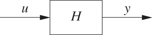
In Chapter 20, we saw that, in the frequency domain, a system’s dynamic response y(s) to an external input u(s) is given by the product of the system’s transfer function H(s) and the input^[22]

y(s) = H(s)u(s)

We can express this equation as a block diagram, where the system (described by its transfer function H) transforms the input u to the output y:

Obviously, we can combine several such systems in series, with the output of one serving as input to the next:

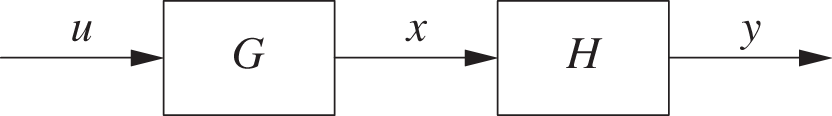
The output of this composite system is the product of its components:

y(s) = H(s) G(s) u(s)

This follows simply because the output of the first element is x(s) = G(s) u(s) and because the output of the second component, acting on the output of the first, is y(s) = H(s) x(s). Therefore, the transfer function ...