Chapter 4. Generative Adversarial Networks
In 2014, Ian Goodfellow et al. presented a paper entitled “Generative Adversarial Nets”1 at the Neural Information Processing Systems conference (NeurIPS) in Montreal. The introduction of generative adversarial networks (or GANs, as they are more commonly known) is now regarded as a key turning point in the history of generative modeling, as the core ideas presented in this paper have spawned some of the most successful and impressive generative models ever created.
This chapter will first lay out the theoretical underpinning of GANs, then we will see how to build our own GAN using Keras.
Introduction
Let’s start with a short story to illustrate some of the fundamental concepts used in the GAN training process.
The story of Brickki bricks and the forgers describes the training process of a generative adversarial network.
A GAN is a battle between two adversaries, the generator and the discriminator. The generator tries to convert random noise into observations that look as if they have been sampled from the original dataset, and the discriminator tries to predict whether an observation comes from the original dataset or is one of the generator’s forgeries. Examples of the inputs and outputs to the two networks are shown in Figure 4-2.
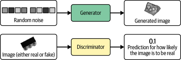
Figure 4-2. Inputs and outputs of the two networks in a GAN
At the start of the process, the generator outputs noisy images and the discriminator predicts randomly. The key to GANs lies in how we alternate the training of the two networks, so that as the generator becomes more adept at fooling the discriminator, the discriminator must adapt in order to maintain its ability to correctly identify which observations are fake. This drives the generator to find new ways to fool the discriminator, and so the cycle continues.
Deep Convolutional GAN (DCGAN)
To see this in action, let’s start building our first GAN in Keras, to generate pictures of bricks.
We will be closely following one of the first major papers on GANs, “Unsupervised Representation Learning with Deep Convolutional Generative Adversarial Networks.”2 In this 2015 paper, the authors show how to build a deep convolutional GAN to generate realistic images from a variety of datasets. They also introduce several changes that significantly improve the quality of the generated images.
Running the Code for This Example
The code for this example can be found in the Jupyter notebook located at notebooks/04_gan/01_dcgan/dcgan.ipynb in the book repository.
The Bricks Dataset
First, you’ll need to download the training data. We’ll be using the Images of LEGO Bricks dataset that is available through Kaggle. This is a computer-rendered collection of 40,000 photographic images of 50 different toy bricks, taken from multiple angles. Some example images of Brickki products are shown in Figure 4-3.

Figure 4-3. Examples of images from the Bricks dataset
You can download the dataset by running the Kaggle dataset downloader script in the book repository, as shown in Example 4-1. This will save the images and accompanying metadata locally to the /data folder.
Example 4-1. Downloading the Bricks dataset
bashscripts/download_kaggle_data.shjoosthazelzetlego-brick-images
We use the Keras function image_dataset_from_directory to create a TensorFlow Dataset pointed at the directory where the images are stored, as shown in Example 4-2. This allows us to read batches of images into memory only when required (e.g., during training), so that we can work with large datasets and not worry about having to fit the entire dataset into memory. It also resizes the images to 64 × 64, interpolating between pixel values.
Example 4-2. Creating a TensorFlow Dataset from image files in a directory
train_data=utils.image_dataset_from_directory("/app/data/lego-brick-images/dataset/",labels=None,color_mode="grayscale",image_size=(64,64),batch_size=128,shuffle=True,seed=42,interpolation="bilinear",)
The original data is scaled in the range [0, 255] to denote the pixel intensity. When training GANs we rescale the data to the range [–1, 1] so that we can use the tanh activation function on the final layer of the generator, which tends to provide stronger gradients than the sigmoid function (Example 4-3).
Example 4-3. Preprocessing the Bricks dataset
defpreprocess(img):img=(tf.cast(img,"float32")-127.5)/127.5returnimgtrain=train_data.map(lambdax:preprocess(x))
Let’s now take a look at how we build the discriminator.
The Discriminator
The goal of the discriminator is to predict if an image is real or fake. This is a supervised image classification problem, so we can use a similar architecture to those we worked with in Chapter 2: stacked convolutional layers, with a single output node.
The full architecture of the discriminator we will be building is shown in Table 4-1.
| Layer (type) | Output shape | Param # |
|---|---|---|
InputLayer |
(None, 64, 64, 1) |
0 |
Conv2D |
(None, 32, 32, 64) |
1,024 |
LeakyReLU |
(None, 32, 32, 64) |
0 |
Dropout |
(None, 32, 32, 64) |
0 |
Conv2D |
(None, 16, 16, 128) |
131,072 |
BatchNormalization |
(None, 16, 16, 128) |
512 |
LeakyReLU |
(None, 16, 16, 128) |
0 |
Dropout |
(None, 16, 16, 128) |
0 |
Conv2D |
(None, 8, 8, 256) |
524,288 |
BatchNormalization |
(None, 8, 8, 256) |
1,024 |
LeakyReLU |
(None, 8, 8, 256) |
0 |
Dropout |
(None, 8, 8, 256) |
0 |
Conv2D |
(None, 4, 4, 512) |
2,097,152 |
BatchNormalization |
(None, 4, 4, 512) |
2,048 |
LeakyReLU |
(None, 4, 4, 512) |
0 |
Dropout |
(None, 4, 4, 512) |
0 |
Conv2D |
(None, 1, 1, 1) |
8,192 |
Flatten |
(None, 1) |
0 |
Total params |
2,765,312 |
Trainable params |
2,763,520 |
Non-trainable params |
1,792 |
The Keras code to build the discriminator is provided in Example 4-4.
Example 4-4. The discriminator
discriminator_input=layers.Input(shape=(64,64,1))x=layers.Conv2D(64,kernel_size=4,strides=2,padding="same",use_bias=False)(discriminator_input)x=layers.LeakyReLU(0.2)(x)x=layers.Dropout(0.3)(x)x=layers.Conv2D(128,kernel_size=4,strides=2,padding="same",use_bias=False)(x)x=layers.BatchNormalization(momentum=0.9)(x)x=layers.LeakyReLU(0.2)(x)x=layers.Dropout(0.3)(x)x=layers.Conv2D(256,kernel_size=4,strides=2,padding="same",use_bias=False)(x)x=layers.BatchNormalization(momentum=0.9)(x)x=layers.LeakyReLU(0.2)(x)x=layers.Dropout(0.3)(x)x=layers.Conv2D(512,kernel_size=4,strides=2,padding="same",use_bias=False)(x)x=layers.BatchNormalization(momentum=0.9)(x)x=layers.LeakyReLU(0.2)(x)x=layers.Dropout(0.3)(x)x=layers.Conv2D(1,kernel_size=4,strides=1,padding="valid",use_bias=False,activation='sigmoid')(x)discriminator_output=layers.Flatten()(x)discriminator=models.Model(discriminator_input,discriminator_output)

Define the
Inputlayer of the discriminator (the image).
Stack
Conv2Dlayers on top of each other, withBatchNormalization,LeakyReLUactivation, andDropoutlayers sandwiched in between.
Flatten the last convolutional layer—by this point, the shape of the tensor is 1 × 1 × 1, so there is no need for a final
Denselayer.
The Keras model that defines the discriminator—a model that takes an input image and outputs a single number between 0 and 1.
Notice how we use a stride of 2 in some of the Conv2D layers to reduce the spatial shape of the tensor as it passes through the network (64 in the original image, then 32, 16, 8, 4, and finally 1), while increasing the number of channels (1 in the grayscale input image, then 64, 128, 256, and finally 512), before collapsing to a single
prediction.
We use a sigmoid activation on the final Conv2D layer to output a number between 0 and 1.
The Generator
Now let’s build the generator. The input to the generator will be a vector drawn from a multivariate standard normal distribution. The output is an image of the same size as an image in the original training data.
This description may remind you of the decoder in a variational autoencoder. In fact, the generator of a GAN fulfills exactly the same purpose as the decoder of a VAE: converting a vector in the latent space to an image. The concept of mapping from a latent space back to the original domain is very common in generative modeling, as it gives us the ability to manipulate vectors in the latent space to change high-level features of images in the original domain.
The architecture of the generator we will be building is shown in Table 4-2.
| Layer (type) | Output shape | Param # |
|---|---|---|
InputLayer |
(None, 100) |
0 |
Reshape |
(None, 1, 1, 100) |
0 |
Conv2DTranspose |
(None, 4, 4, 512) |
819,200 |
BatchNormalization |
(None, 4, 4, 512) |
2,048 |
ReLU |
(None, 4, 4, 512) |
0 |
Conv2DTranspose |
(None, 8, 8, 256) |
2,097,152 |
BatchNormalization |
(None, 8, 8, 256) |
1,024 |
ReLU |
(None, 8, 8, 256) |
0 |
Conv2DTranspose |
(None, 16, 16, 128) |
524,288 |
BatchNormalization |
(None, 16, 16, 128) |
512 |
ReLU |
(None, 16, 16, 128) |
0 |
Conv2DTranspose |
(None, 32, 32, 64) |
131,072 |
BatchNormalization |
(None, 32, 32, 64) |
256 |
ReLU |
(None, 32, 32, 64) |
0 |
Conv2DTranspose |
(None, 64, 64, 1) |
1,024 |
Total params |
3,576,576 |
Trainable params |
3,574,656 |
Non-trainable params |
1,920 |
The code for building the generator is given in Example 4-5.
Example 4-5. The generator
generator_input=layers.Input(shape=(100,))x=layers.Reshape((1,1,100))(generator_input)x=layers.Conv2DTranspose(512,kernel_size=4,strides=1,padding="valid",use_bias=False)(x)x=layers.BatchNormalization(momentum=0.9)(x)x=layers.LeakyReLU(0.2)(x)x=layers.Conv2DTranspose(256,kernel_size=4,strides=2,padding="same",use_bias=False)(x)x=layers.BatchNormalization(momentum=0.9)(x)x=layers.LeakyReLU(0.2)(x)x=layers.Conv2DTranspose(128,kernel_size=4,strides=2,padding="same",use_bias=False)(x)x=layers.BatchNormalization(momentum=0.9)(x)x=layers.LeakyReLU(0.2)(x)x=layers.Conv2DTranspose(64,kernel_size=4,strides=2,padding="same",use_bias=False)(x)x=layers.BatchNormalization(momentum=0.9)(x)x=layers.LeakyReLU(0.2)(x)generator_output=layers.Conv2DTranspose(1,kernel_size=4,strides=2,padding="same",use_bias=False,activation='tanh')(x)generator=models.Model(generator_input,generator_output)

Define the
Inputlayer of the generator—a vector of length 100.
We use a
Reshapelayer to give a 1 × 1 × 100 tensor, so that we can start applying convolutional transpose operations.
We pass this through four
Conv2DTransposelayers, withBatchNormalizationandLeakyReLUlayers sandwiched in between.
The final
Conv2DTransposelayer uses a tanh activation function to transform the output to the range [–1, 1], to match the original image domain.
The Keras model that defines the generator—a model that accepts a vector of length 100 and outputs a tensor of shape
[64, 64, 1].
Notice how we use a stride of 2 in some of the Conv2DTranspose layers to increase the spatial shape of the tensor as it passes through the network (1 in the original vector, then 4, 8, 16, 32, and finally 64), while decreasing the number of channels (512 then 256, 128, 64, and finally 1 to match the grayscale output).
Training the DCGAN
As we have seen, the architectures of the generator and discriminator in a DCGAN are very simple and not so different from the VAE models that we looked at in Chapter 3. The key to understanding GANs lies in understanding the training process for the generator and discriminator.
We can train the discriminator by creating a training set where some of the images are real observations from the training set and some are fake outputs from the generator. We then treat this as a supervised learning problem, where the labels are 1 for the real images and 0 for the fake images, with binary cross-entropy as the loss function.
How should we train the generator? We need to find a way of scoring each generated image so that it can optimize toward high-scoring images. Luckily, we have a discriminator that does exactly that! We can generate a batch of images and pass these through the discriminator to get a score for each image. The loss function for the generator is then simply the binary cross-entropy between these probabilities and a vector of ones, because we want to train the generator to produce images that the discriminator thinks are real.
Crucially, we must alternate the training of these two networks, making sure that we only update the weights of one network at a time. For example, during the generator training process, only the generator’s weights are updated. If we allowed the discriminator’s weights to change as well, the discriminator would just adjust so that it is more likely to predict the generated images to be real, which is not the desired outcome. We want generated images to be predicted close to 1 (real) because the generator is strong, not because the discriminator is weak.
A diagram of the training process for the discriminator and generator is shown in Figure 4-5.
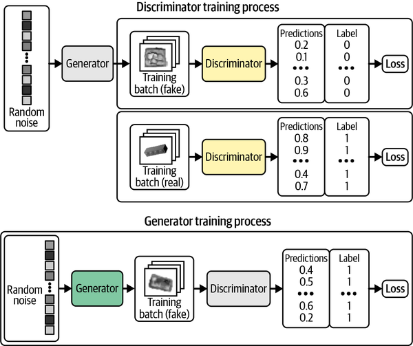
Figure 4-5. Training the DCGAN—gray boxes indicate that the weights are frozen during training
Keras provides us with the ability to create a custom train_step function to implement this logic. Example 4-7 shows the full DCGAN model class.
Example 4-7. Compiling the DCGAN
classDCGAN(models.Model):def__init__(self,discriminator,generator,latent_dim):super(DCGAN,self).__init__()self.discriminator=discriminatorself.generator=generatorself.latent_dim=latent_dimdefcompile(self,d_optimizer,g_optimizer):super(DCGAN,self).compile()self.loss_fn=losses.BinaryCrossentropy()self.d_optimizer=d_optimizerself.g_optimizer=g_optimizerself.d_loss_metric=metrics.Mean(name="d_loss")self.g_loss_metric=metrics.Mean(name="g_loss")@propertydefmetrics(self):return[self.d_loss_metric,self.g_loss_metric]deftrain_step(self,real_images):batch_size=tf.shape(real_images)[0]random_latent_vectors=tf.random.normal(shape=(batch_size,self.latent_dim))withtf.GradientTape()asgen_tape,tf.GradientTape()asdisc_tape:generated_images=self.generator(random_latent_vectors,training=True)real_predictions=self.discriminator(real_images,training=True)fake_predictions=self.discriminator(generated_images,training=True)real_labels=tf.ones_like(real_predictions)real_noisy_labels=real_labels+0.1*tf.random.uniform(tf.shape(real_predictions))fake_labels=tf.zeros_like(fake_predictions)fake_noisy_labels=fake_labels-0.1*tf.random.uniform(tf.shape(fake_predictions))d_real_loss=self.loss_fn(real_noisy_labels,real_predictions)d_fake_loss=self.loss_fn(fake_noisy_labels,fake_predictions)d_loss=(d_real_loss+d_fake_loss)/2.0g_loss=self.loss_fn(real_labels,fake_predictions)gradients_of_discriminator=disc_tape.gradient(d_loss,self.discriminator.trainable_variables)gradients_of_generator=gen_tape.gradient(g_loss,self.generator.trainable_variables)self.d_optimizer.apply_gradients(zip(gradients_of_discriminator,discriminator.trainable_variables))self.g_optimizer.apply_gradients(zip(gradients_of_generator,generator.trainable_variables))self.d_loss_metric.update_state(d_loss)self.g_loss_metric.update_state(g_loss)return{m.name:m.result()forminself.metrics}dcgan=DCGAN(discriminator=discriminator,generator=generator,latent_dim=100)dcgan.compile(d_optimizer=optimizers.Adam(learning_rate=0.0002,beta_1=0.5,beta_2=0.999),g_optimizer=optimizers.Adam(learning_rate=0.0002,beta_1=0.5,beta_2=0.999),)dcgan.fit(train,epochs=300)

The loss function for the generator and discriminator is
BinaryCrossentropy.
To train the network, first sample a batch of vectors from a multivariate standard normal distribution.

Next, pass these through the generator to produce a batch of generated images.

Now ask the discriminator to predict the realness of the batch of real images…

…and the batch of generated images.

The discriminator loss is the average binary cross-entropy across both the real images (with label 1) and the fake images (with label 0).

The generator loss is the binary cross-entropy between the discriminator predictions for the generated images and a label of 1.

Update the weights of the discriminator and generator separately.
The discriminator and generator are constantly fighting for dominance, which can make the DCGAN training process unstable. Ideally, the training process will find an equilibrium that allows the generator to learn meaningful information from the discriminator and the quality of the images will start to improve. After enough epochs, the discriminator tends to end up dominating, as shown in Figure 4-6, but this may not be a problem as the generator may have already learned to produce sufficiently high-quality images by this point.
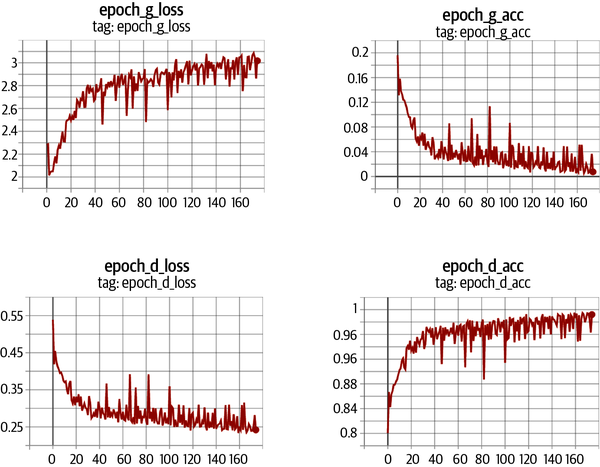
Figure 4-6. Loss and accuracy of the discriminator and generator during training
Adding Noise to the Labels
A useful trick when training GANs is to add a small amount of random noise to the training labels. This helps to improve the stability of the training process and sharpen the generated images. This label smoothing acts as way to tame the discriminator, so that it is presented with a more challenging task and doesn’t overpower the generator.
Analysis of the DCGAN
By observing images produced by the generator at specific epochs during training (Figure 4-7), it is clear that the generator is becoming increasingly adept at producing images that could have been drawn from the training set.
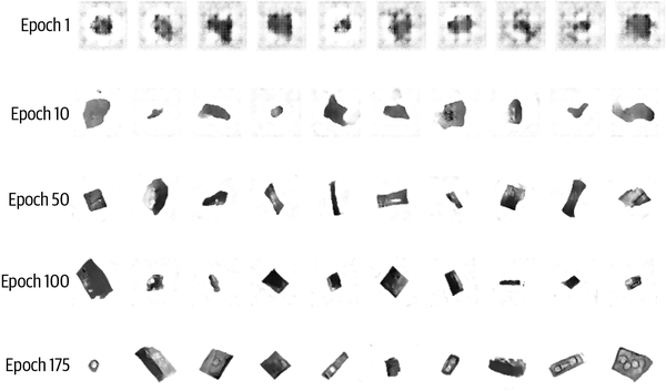
Figure 4-7. Output from the generator at specific epochs during training
It is somewhat miraculous that a neural network is able to convert random noise into something meaningful. It is worth remembering that we haven’t provided the model with any additional features beyond the raw pixels, so it has to work out high-level concepts such as how to draw shadows, cuboids, and circles entirely by itself.
Another requirement of a successful generative model is that it doesn’t only reproduce images from the training set. To test this, we can find the image from the training set that is closest to a particular generated example. A good measure for distance is the L1 distance, defined as:
def compare_images(img1, img2):
    return np.mean(np.abs(img1 - img2))
Figure 4-8 shows the closest observations in the training set for a selection of generated images. We can see that while there is some degree of similarity between the generated images and the training set, they are not identical. This shows that the generator has understood these high-level features and can generate examples that are distinct from those it has already seen.
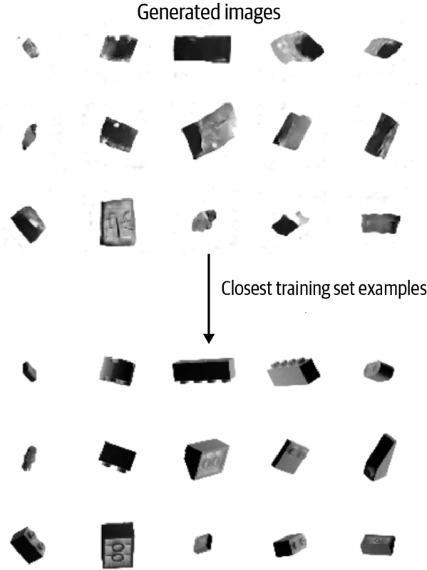
Figure 4-8. Closest matches of generated images from the training set
GAN Training: Tips and Tricks
While GANs are a major breakthrough for generative modeling, they are also notoriously difficult to train. We will explore some of the most common problems and challenges encountered when training GANs in this section, alongside potential solutions. In the next section, we will look at some more fundamental adjustments to the GAN framework that we can make to remedy many of these problems.
Discriminator overpowers the generator
If the discriminator becomes too strong, the signal from the loss function becomes too weak to drive any meaningful improvements in the generator. In the worst-case scenario, the discriminator perfectly learns to separate real images from fake images and the gradients vanish completely, leading to no training whatsoever, as can be seen in Figure 4-9.
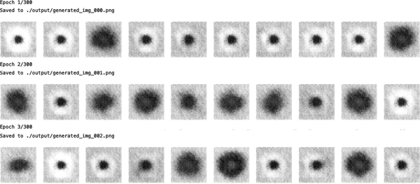
Figure 4-9. Example output when the discriminator overpowers the generator
If you find your discriminator loss function collapsing, you need to find ways to weaken the discriminator. Try the following suggestions:
-
Increase the
rateparameter of theDropoutlayers in the discriminator to dampen the amount of information that flows through the network. -
Reduce the learning rate of the discriminator.
-
Reduce the number of convolutional filters in the discriminator.
-
Add noise to the labels when training the discriminator.
-
Flip the labels of some images at random when training the discriminator.
Generator overpowers the discriminator
If the discriminator is not powerful enough, the generator will find ways to easily trick the discriminator with a small sample of nearly identical images. This is known as mode collapse.
For example, suppose we were to train the generator over several batches without updating the discriminator in between. The generator would be inclined to find a single observation (also known as a mode) that always fools the discriminator and would start to map every point in the latent input space to this image. Moreover, the gradients of the loss function would collapse to near 0, so it wouldn’t be able to recover from this state.
Even if we then tried to retrain the discriminator to stop it being fooled by this one point, the generator would simply find another mode that fools the discriminator, since it has already become numb to its input and therefore has no incentive to diversify its output.
The effect of mode collapse can be seen in Figure 4-10.
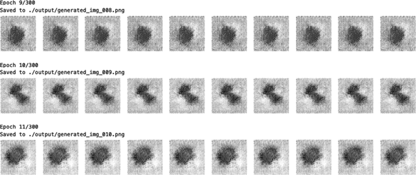
Figure 4-10. Example of mode collapse when the generator overpowers the discriminator
If you find that your generator is suffering from mode collapse, you can try strengthening the discriminator using the opposite suggestions to those listed in the previous section. Also, you can try reducing the learning rate of both networks and increasing the batch size.
Uninformative loss
Since the deep learning model is compiled to minimize the loss function, it would be natural to think that the smaller the loss function of the generator, the better the quality of the images produced. However, since the generator is only graded against the current discriminator and the discriminator is constantly improving, we cannot compare the loss function evaluated at different points in the training process. Indeed, in Figure 4-6, the loss function of the generator actually increases over time, even though the quality of the images is clearly improving. This lack of correlation between the generator loss and image quality sometimes makes GAN training difficult to monitor.
Hyperparameters
As we have seen, even with simple GANs, there are a large number of hyperparameters to tune. As well as the overall architecture of both the discriminator and the generator, there are the parameters that govern batch normalization, dropout, learning rate, activation layers, convolutional filters, kernel size, striding, batch size, and latent space size to consider. GANs are highly sensitive to very slight changes in all of these parameters, and finding a set of parameters that works is often a case of educated trial and error, rather than following an established set of guidelines.
This is why it is important to understand the inner workings of the GAN and know how to interpret the loss function—so that you can identify sensible adjustments to the hyperparameters that might improve the stability of the model.
Tackling GAN challenges
In recent years, several key advancements have drastically improved the overall stability of GAN models and diminished the likelihood of some of the problems listed earlier, such as mode collapse.
In the remainder of this chapter we shall examine the Wasserstein GAN with Gradient Penalty (WGAN-GP), which makes several key adjustments to the GAN framework we have explored thus far to improve the stability and quality of the image generation process.
Wasserstein GAN with Gradient Penalty (WGAN-GP)
In this section we will build a WGAN-GP to generate faces from the CelebA dataset that we utilized in Chapter 3.
Running the Code for This Example
The code for this example can be found in the Jupyter notebook located at notebooks/04_gan/02_wgan_gp/wgan_gp.ipynb in the book repository.
The code has been adapted from the excellent WGAN-GP tutorial created by Aakash Kumar Nain, available on the Keras website.
The Wasserstein GAN (WGAN), introduced in a 2017 paper by Arjovsky et al.,4 was one of the first big steps toward stabilizing GAN training. With a few changes, the authors were able to show how to train GANs that have the following two properties (quoted from the paper):
-
A meaningful loss metric that correlates with the generator’s convergence and sample quality
-
Improved stability of the optimization process
Specifically, the paper introduces the Wasserstein loss function for both the discriminator and the generator. Using this loss function instead of binary cross-entropy results in a more stable convergence of the GAN.
In this section we’ll define the Wasserstein loss function and then see what other changes we need to make to the model architecture and training process to incorporate our new loss function.
You can find the full model class in the Jupyter notebook located at chapter05/wgan-gp/faces/train.ipynb in the book repository.
Wasserstein Loss
Let’s first remind ourselves of the definition of binary cross-entropy loss—the function that we are currently using to train the discriminator and generator of the GAN (Equation 4-1).
Equation 4-1. Binary cross-entropy loss
To train the GAN discriminator , we calculate the loss when comparing predictions for real images to the response and predictions for generated images to the response . Therefore, for the GAN discriminator, minimizing the loss function can be written as shown in Equation 4-2.
Equation 4-2. GAN discriminator loss minimization
To train the GAN generator , we calculate the loss when comparing predictions for generated images to the response . Therefore, for the GAN generator, minimizing the loss function can be written as shown in Equation 4-3.
Equation 4-3. GAN generator loss minimization
Now let’s compare this to the Wasserstein loss function.
First, the Wasserstein loss requires that we use and = –1 as labels, rather than 1 and 0. We also remove the sigmoid activation from the final layer of the discriminator, so that predictions are no longer constrained to fall in the range [0, 1] but instead can now be any number in the range (, ). For this reason, the discriminator in a WGAN is usually referred to as a critic that outputs a score rather than a probability.
The Wasserstein loss function is defined as follows:
To train the WGAN critic , we calculate the loss when comparing predictions for real images to the response and predictions for generated images to the response = –1. Therefore, for the WGAN critic, minimizing the loss function can be written as follows:
In other words, the WGAN critic tries to maximize the difference between its predictions for real images and generated images.
To train the WGAN generator, we calculate the loss when comparing predictions for generated images to the response . Therefore, for the WGAN generator, minimizing the loss function can be written as follows:
In other words, the WGAN generator tries to produce images that are scored as highly as possible by the critic (i.e., the critic is fooled into thinking they are real).
The Lipschitz Constraint
It may surprise you that we are now allowing the critic to output any number in the range (, ), rather than applying a sigmoid function to restrict the output to the usual [0, 1] range. The Wasserstein loss can therefore be very large, which is unsettling—usually, large numbers in neural networks are to be avoided!
In fact, the authors of the WGAN paper show that for the Wasserstein loss function to work, we also need to place an additional constraint on the critic. Specifically, it is required that the critic is a 1-Lipschitz continuous function. Let’s pick this apart to understand what it means in more detail.
The critic is a function that converts an image into a prediction. We say that this function is 1-Lipschitz if it satisfies the following inequality for any two input images, and :
Here, is the average pixelwise absolute difference between two images and is the absolute difference between the critic predictions. Essentially, we require a limit on the rate at which the predictions of the critic can change between two images (i.e., the absolute value of the gradient must be at most 1 everywhere). We can see this applied to a Lipschitz continuous 1D function in Figure 4-11—at no point does the line enter the cone, wherever you place the cone on the line. In other words, there is a limit on the rate at which the line can rise or fall at any point.

Figure 4-11. A Lipschitz continuous function (source: Wikipedia)
Tip
For those who want to delve deeper into the mathematical rationale behind why the Wasserstein loss only works when this constraint is enforced, Jonathan Hui offers an excellent explanation.
Enforcing the Lipschitz Constraint
In the original WGAN paper, the authors show how it is possible to enforce the Lipschitz constraint by clipping the weights of the critic to lie within a small range, [–0.01, 0.01], after each training batch.
One of the criticisms of this approach is that the capacity of the critic to learn is greatly diminished, since we are clipping its weights. In fact, even in the original WGAN paper the authors write, “Weight clipping is a clearly terrible way to enforce a Lipschitz constraint.” A strong critic is pivotal to the success of a WGAN, since without accurate gradients, the generator cannot learn how to adapt its weights to produce better samples.
Therefore, other researchers have looked for alternative ways to enforce the Lipschitz constraint and improve the capacity of the WGAN to learn complex features. One such method is the Wasserstein GAN with Gradient Penalty.
In the paper introducing this variant,5 the authors show how the Lipschitz constraint can be enforced directly by including a gradient penalty term in the loss function for the critic that penalizes the model if the gradient norm deviates from 1. This results in a far more stable training process.
In the next section, we’ll see how to build this extra term into the loss function for our critic.
The Gradient Penalty Loss
Figure 4-12 is a diagram of the training process for the critic of a WGAN-GP. If we compare this to the original discriminator training process from Figure 4-5, we can see that the key addition is the gradient penalty loss included as part of the overall loss function, alongside the Wasserstein loss from the real and fake images.
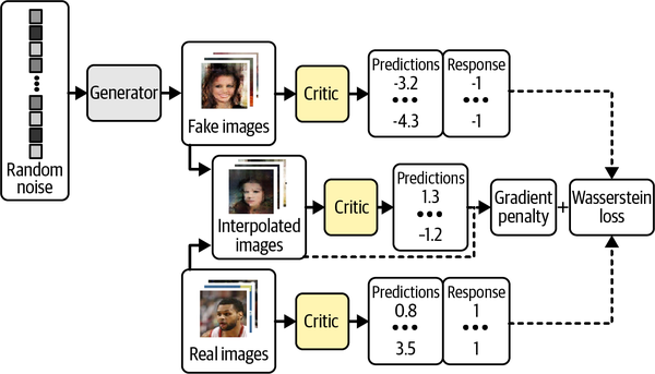
Figure 4-12. The WGAN-GP critic training process
The gradient penalty loss measures the squared difference between the norm of the gradient of the predictions with respect to the input images and 1. The model will naturally be inclined to find weights that ensure the gradient penalty term is minimized, thereby encouraging the model to conform to the Lipschitz constraint.
It is intractable to calculate this gradient everywhere during the training process, so instead the WGAN-GP evaluates the gradient at only a handful of points. To ensure a balanced mix, we use a set of interpolated images that lie at randomly chosen points along lines connecting the batch of real images to the batch of fake images pairwise, as shown in Figure 4-13.
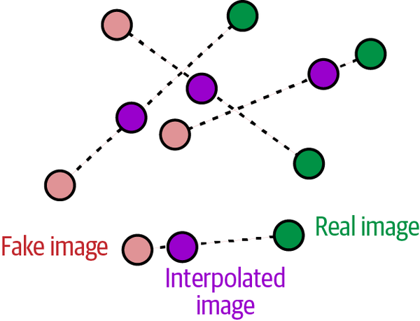
Figure 4-13. Interpolating between images
In Example 4-8, we show how the gradient penalty is calculated in code.
Example 4-8. The gradient penalty loss function
defgradient_penalty(self,batch_size,real_images,fake_images):alpha=tf.random.normal([batch_size,1,1,1],0.0,1.0)diff=fake_images-real_imagesinterpolated=real_images+alpha*diffwithtf.GradientTape()asgp_tape:gp_tape.watch(interpolated)pred=self.critic(interpolated,training=True)grads=gp_tape.gradient(pred,[interpolated])[0]norm=tf.sqrt(tf.reduce_sum(tf.square(grads),axis=[1,2,3]))gp=tf.reduce_mean((norm-1.0)**2)returngp

Each image in the batch gets a random number, between 0 and 1, stored as the vector
alpha.
A set of interpolated images is calculated.

The critic is asked to score each of these interpolated images.

The gradient of the predictions is calculated with respect to the input images.

The L2 norm of this vector is calculated.

The function returns the average squared distance between the L2 norm and 1.
Training the WGAN-GP
A key benefit of using the Wasserstein loss function is that we no longer need to worry about balancing the training of the critic and the generator—in fact, when using the Wasserstein loss, the critic must be trained to convergence before updating the generator, to ensure that the gradients for the generator update are accurate. This is in contrast to a standard GAN, where it is important not to let the discriminator get too strong.
Therefore, with Wasserstein GANs, we can simply train the critic several times between generator updates, to ensure it is close to convergence. A typical ratio used is three to five critic updates per generator update.
We have now introduced both of the key concepts behind the WGAN-GP—the Wasserstein loss and the gradient penalty term that is included in the critic loss function. The training step of the WGAN model that incorporates all of these ideas is shown in Example 4-9.
Example 4-9. Training the WGAN-GP
deftrain_step(self,real_images):batch_size=tf.shape(real_images)[0]foriinrange(3):random_latent_vectors=tf.random.normal(shape=(batch_size,self.latent_dim))withtf.GradientTape()astape:fake_images=self.generator(random_latent_vectors,training=True)fake_predictions=self.critic(fake_images,training=True)real_predictions=self.critic(real_images,training=True)c_wass_loss=tf.reduce_mean(fake_predictions)-tf.reduce_mean(real_predictions)c_gp=self.gradient_penalty(batch_size,real_images,fake_images)c_loss=c_wass_loss+c_gp*self.gp_weightc_gradient=tape.gradient(c_loss,self.critic.trainable_variables)self.c_optimizer.apply_gradients(zip(c_gradient,self.critic.trainable_variables))random_latent_vectors=tf.random.normal(shape=(batch_size,self.latent_dim))withtf.GradientTape()astape:fake_images=self.generator(random_latent_vectors,training=True)fake_predictions=self.critic(fake_images,training=True)g_loss=-tf.reduce_mean(fake_predictions)gen_gradient=tape.gradient(g_loss,self.generator.trainable_variables)self.g_optimizer.apply_gradients(zip(gen_gradient,self.generator.trainable_variables))self.c_loss_metric.update_state(c_loss)self.c_wass_loss_metric.update_state(c_wass_loss)self.c_gp_metric.update_state(c_gp)self.g_loss_metric.update_state(g_loss)return{m.name:m.result()forminself.metrics}

Perform three critic updates.

Calculate the Wasserstein loss for the critic—the difference between the average prediction for the fake images and the real images.

Calculate the gradient penalty term (see Example 4-8).

The critic loss function is a weighted sum of the Wasserstein loss and the gradient penalty.

Update the weights of the critic.

Calculate the Wasserstein loss for the generator.

Update the weights of the generator.
Batch Normalization in a WGAN-GP
One last consideration we should note before training a WGAN-GP is that batch normalization shouldn’t be used in the critic. This is because batch normalization creates correlation between images in the same batch, which makes the gradient penalty loss less effective. Experiments have shown that WGAN-GPs can still produce excellent results even without batch normalization in the critic.
We have now covered all of the key differences between a standard GAN and a WGAN-GP. To recap:
-
A WGAN-GP uses the Wasserstein loss.
-
The WGAN-GP is trained using labels of 1 for real and –1 for fake.
-
There is no sigmoid activation in the final layer of the critic.
-
Include a gradient penalty term in the loss function for the critic.
-
Train the critic multiple times for each update of the generator.
-
There are no batch normalization layers in the critic.
Analysis of the WGAN-GP
Let’s take a look at some example outputs from the generator, after 25 epochs of training (Figure 4-14).
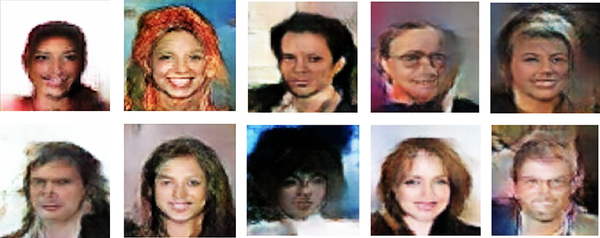
Figure 4-14. WGAN-GP face examples
The model has learned the significant high-level attributes of a face, and there is no sign of mode collapse.
We can also see how the loss functions of the model evolve over time (Figure 4-15)—the loss functions of both the critic and generator are highly stable and convergent.
If we compare the WGAN-GP output to the VAE output from the previous chapter, we can see that the GAN images are generally sharper—especially the definition between the hair and the background. This is true in general; VAEs tend to produce softer images that blur color boundaries, whereas GANs are known to produce sharper, more well-defined images.
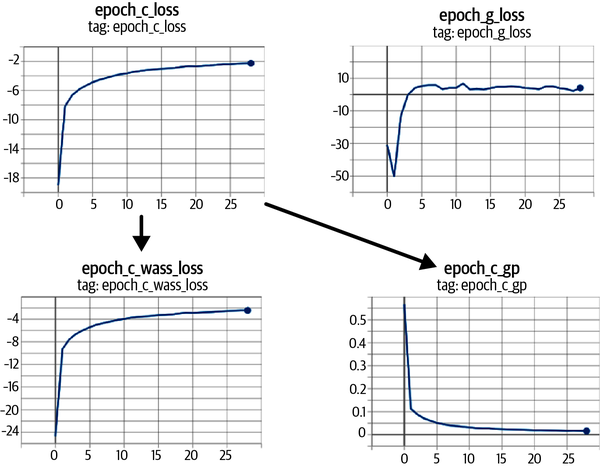
Figure 4-15. WGAN-GP loss curves: the critic loss (epoch_c_loss) is broken down into the Wasserstein loss (epoch_c_wass) and the gradient penalty loss (epoch_c_gp)
It is also true that GANs are generally more difficult to train than VAEs and take longer to reach a satisfactory quality. However, many state-of-the-art generative models today are GAN-based, as the rewards for training large-scale GANs on GPUs over a longer period of time are significant.
Conditional GAN (CGAN)
So far in this chapter, we have built GANs that are able to generate realistic images from a given training set. However, we haven’t been able to control the type of image we would like to generate—for example, a male or female face, or a large or small brick. We can sample a random point from the latent space, but we do not have the ability to easily understand what kind of image will be produced given the choice of latent variable.
In the final part of this chapter we shall turn our attention to building a GAN where we are able to control the output—a so called conditional GAN. This idea, first introduced in “Conditional Generative Adversarial Nets” by Mirza and Osindero in 2014,6 is a relatively simple extension to the GAN architecture.
Running the Code for This Example
The code for this example can be found in the Jupyter notebook located at notebooks/04_gan/03_cgan/cgan.ipynb in the book repository.
The code has been adapted from the excellent CGAN tutorial created by Sayak Paul, available on the Keras website.
CGAN Architecture
In this example, we will condition our CGAN on the blond hair attribute of the faces dataset. That is, we will be able to explicitly specify whether we want to generate an image with blond hair or not. This label is provided as part of the CelebA dataset.
The high-level CGAN architecture is shown in Figure 4-16.
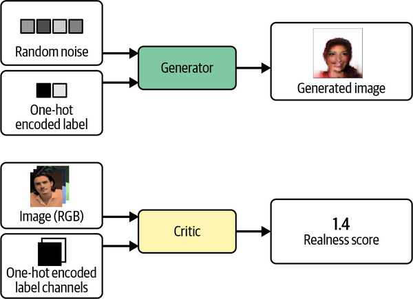
Figure 4-16. Inputs and outputs of the generator and critic in a CGAN
The key difference between a standard GAN and a CGAN is that in a CGAN we pass in extra information to the generator and critic relating to the label. In the generator, this is simply appended to the latent space sample as a one-hot encoded vector. In the critic, we add the label information as extra channels to the RGB image. We do this by repeating the one-hot encoded vector to fill the same shape as the input images.
CGANs work because the critic now has access to extra information regarding the content of the image, so the generator must ensure that its output agrees with the provided label, in order to keep fooling the critic. If the generator produced perfect images that disagreed with the image label the critic would be able to tell that they were fake simply because the images and labels did not match.
Tip
In our example, our one-hot encoded label will have length 2, because there are two classes (Blonde and Not Blond). However, you can have as many labels as you like—for example, you could train a CGAN on the Fashion-MNIST dataset to output one of the 10 different fashion items, by incorporating a one-hot encoded label vector of length 10 into the input of the generator and 10 additional one-hot encoded label channels into the input of the critic.
The only change we need to make to the architecture is to concatenate the label information to the existing inputs of the generator and the critic, as shown in Example 4-10.
Example 4-10. Input layers in the CGAN
critic_input=layers.Input(shape=(64,64,3))label_input=layers.Input(shape=(64,64,2))x=layers.Concatenate(axis=-1)([critic_input,label_input])...generator_input=layers.Input(shape=(32,))label_input=layers.Input(shape=(2,))x=layers.Concatenate(axis=-1)([generator_input,label_input])x=layers.Reshape((1,1,34))(x)...
Training the CGAN
We must also make some changes to the train_step of the CGAN to match the new input formats of the generator and critic, as shown in Example 4-11.
Example 4-11. The train_step of the CGAN
deftrain_step(self,data):real_images,one_hot_labels=dataimage_one_hot_labels=one_hot_labels[:,None,None,:]image_one_hot_labels=tf.repeat(image_one_hot_labels,repeats=64,axis=1)image_one_hot_labels=tf.repeat(image_one_hot_labels,repeats=64,axis=2)batch_size=tf.shape(real_images)[0]foriinrange(self.critic_steps):random_latent_vectors=tf.random.normal(shape=(batch_size,self.latent_dim))withtf.GradientTape()astape:fake_images=self.generator([random_latent_vectors,one_hot_labels],training=True)fake_predictions=self.critic([fake_images,image_one_hot_labels],training=True)real_predictions=self.critic([real_images,image_one_hot_labels],training=True)c_wass_loss=tf.reduce_mean(fake_predictions)-tf.reduce_mean(real_predictions)c_gp=self.gradient_penalty(batch_size,real_images,fake_images,image_one_hot_labels)c_loss=c_wass_loss+c_gp*self.gp_weightc_gradient=tape.gradient(c_loss,self.critic.trainable_variables)self.c_optimizer.apply_gradients(zip(c_gradient,self.critic.trainable_variables))random_latent_vectors=tf.random.normal(shape=(batch_size,self.latent_dim))withtf.GradientTape()astape:fake_images=self.generator([random_latent_vectors,one_hot_labels],training=True)fake_predictions=self.critic([fake_images,image_one_hot_labels],training=True)g_loss=-tf.reduce_mean(fake_predictions)gen_gradient=tape.gradient(g_loss,self.generator.trainable_variables)self.g_optimizer.apply_gradients(zip(gen_gradient,self.generator.trainable_variables))

The images and labels are unpacked from the input data.

The one-hot encoded vectors are expanded to one-hot encoded images that have the same spatial size as the input images (64 × 64).

The generator is now fed with a list of two inputs—the random latent vectors and the one-hot encoded label vectors.

The critic is now fed with a list of two inputs—the fake/real images and the one-hot encoded label channels.

The gradient penalty function also requires the one-hot encoded label channels to be passed through as it uses the critic.

The changes made to the critic training step also apply to the generator training step.
Analysis of the CGAN
We can control the CGAN output by passing a particular one-hot encoded label into the input of the generator. For example, to generate a face with nonblond hair, we pass in the vector [1, 0]. To generate a face with blond hair, we pass in the vector [0, 1].
The output from the CGAN can be seen in Figure 4-17. Here, we keep the random latent vectors the same across the examples and change only the conditional label vector. It is clear that the CGAN has learned to use the label vector to control only the hair color attribute of the images. It is impressive that the rest of the image barely changes—this is proof that GANs are able to organize points in the latent space in such a way that individual features can be decoupled from each other.
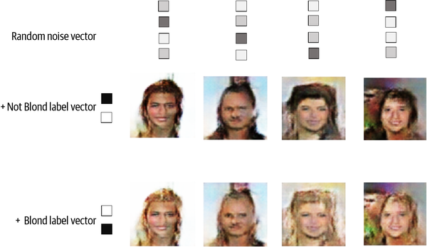
Figure 4-17. Output from the CGAN when the Blond and Not Blond vectors are appended to the latent sample
Tip
If labels are available for your dataset, it is generally a good idea to include them as input to your GAN even if you do not necessarily need to condition the generated output on the label, as they tend to improve the quality of images generated. You can think of the labels as just a highly informative extension to the pixel input.
Summary
In this chapter we explored three different generative adversarial network (GAN) models: the deep convolutional GAN (DCGAN), the more sophisticated Wasserstein GAN with Gradient Penalty (WGAN-GP), and the conditional GAN (CGAN).
All GANs are characterized by a generator versus discriminator (or critic) architecture, with the discriminator trying to “spot the difference” between real and fake images and the generator aiming to fool the discriminator. By balancing how these two adversaries are trained, the GAN generator can gradually learn how to produce similar observations to those in the training set.
We first saw how to train a DCGAN to generate images of toy bricks. It was able to learn how to realistically represent 3D objects as images, including accurate representations of shadow, shape, and texture. We also explored the different ways in which GAN training can fail, including mode collapse and vanishing gradients.
We then explored how the Wasserstein loss function remedied many of these problems and made GAN training more predictable and reliable. The WGAN-GP places the 1-Lipschitz requirement at the heart of the training process by including a term in the loss function to pull the gradient norm toward 1.
We applied the WGAN-GP to the problem of face generation and saw how by simply choosing points from a standard normal distribution, we can generate new faces. This sampling process is very similar to a VAE, though the faces produced by a GAN are quite different—often sharper, with greater distinction between different parts of the image.
Finally, we built a CGAN that allowed us to control the type of image that is generated. This works by passing in the label as input to the critic and generator, thereby giving the network the additional information it needs in order to condition the generated output on a given label.
Overall, we have seen how the GAN framework is extremely flexible and able to be adapted to many interesting problem domains. In particular, GANs have driven significant progress in the field of image generation with many interesting extensions to the underlying framework, as we shall see in Chapter 10.
In the next chapter, we will explore a different family of generative model that is ideal for modeling sequential data—autoregressive models.
1 Ian J. Goodfellow et al., “Generative Adversarial Nets,” June 10, 2014, https://arxiv.org/abs/1406.2661
2 Alec Radford et al., “Unsupervised Representation Learning with Deep Convolutional Generative Adversarial Networks,” January 7, 2016, https://arxiv.org/abs/1511.06434.
3 Augustus Odena et al., “Deconvolution and Checkerboard Artifacts,” October 17, 2016, https://distill.pub/2016/deconv-checkerboard.
4 Martin Arjovsky et al., “Wasserstein GAN,” January 26, 2017, https://arxiv.org/abs/1701.07875.
5 Ishaan Gulrajani et al., “Improved Training of Wasserstein GANs,” March 31, 2017, https://arxiv.org/abs/1704.00028.
6 Mehdi Mirza and Simon Osindero, “Conditional Generative Adversarial Nets,” November 6, 2014, https://arxiv.org/abs/1411.1784.
Get Generative Deep Learning, 2nd Edition now with the O’Reilly learning platform.
O’Reilly members experience books, live events, courses curated by job role, and more from O’Reilly and nearly 200 top publishers.

