Graph Databases

Chapter 4. Building a Graph Database Application

In this chapter we discuss some of the practical issues of working with a graph database. In previous chapters we’ve looked at graph data; in this chapter, we’ll apply that knowledge in the context of developing a graph database application. We’ll look at some of the data modeling questions that may arise, and at some of the application architecture choices available to us.

In our experience, graph database applications are highly amenable to being developed using the evolutionary, incremental, and iterative software development practices in widespread use today. A key feature of these practices is the prevalence of testing throughout the software development life cycle. Here we’ll show how we develop our data model and our application in a test-driven fashion.

At the end of the chapter, we’ll look at some of the issues we’ll need to consider when planning for production.

Data Modeling

We covered modeling and working with graph data in detail in Chapter 3. Here we summarize some of the more important modeling guidelines, and discuss how implementing a graph data model fits with iterative and incremental software development techniques.

Describe the Model in Terms of the Application’s Needs

The questions we need to ask of the data help identify entities and relationships. Agile user stories provide a concise means for expressing an outside-in, user-centered view of an application’s needs, and the questions that arise in the course of satisfying this need.^[6] Here’s an example of a user story for a book review web application:

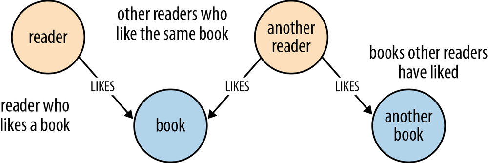
AS A reader who likes a book, I WANT to know which books other readers who like the same book have liked, SO THAT I can find other books to read.

This story expresses a user need, which motivates the shape and content of our data model. From a data modeling point of view, the AS A clause establishes a context comprising two entities—a reader and a book—plus the LIKES relationship that connects them. The I WANT clause then poses a question: which books have the readers who like the book I’m currently reading also liked? This question exposes more LIKES relationships, and more entities: other readers and other books.

The entities and relationships that we’ve surfaced in analyzing the user story quickly translate into a simple data model, as shown in Figure 4-1.

Figure 4-1. Data model for the book reviews user story

Because this data model directly encodes the question presented by the user story, it lends itself to being queried in a way that similarly reflects the structure of the question we want to ask of the data:

START reader=node:users(name={readerName})
      book=node:books(isbn={bookISBN})
MATCH reader-[:LIKES]->book<-[:LIKES]-other_readers-[:LIKES]->books
RETURN books.title

Nodes for Things, Relationships for Structure

Though not applicable in every situation, these general guidelines will help us choose when to use nodes, and when to use relationships:

• Use nodes to represent entities—that is, the things that are of interest to us in our domain.
• Use relationships both to express the connections between entities and to establish semantic context for each entity, thereby structuring the domain.
• Use relationship direction to further clarify relationship semantics. Many relationships are asymmetrical, which is why relationships in a property graph are always directed. For bidirectional relationships, we should make our queries ignore direction.
• Use node properties to represent entity attributes, plus any necessary entity metadata, such as timestamps, version numbers, etc.
• Use relationship properties to express the strength, weight, or quality of a relationship, plus any necessary relationship metadata, such as timestamps, version numbers, etc.

It pays to be diligent about discovering and capturing domain entities. As we saw in Chapter 3, it’s relatively easy to model things that really ought to be represented as nodes using sloppily named relationships instead. If we’re tempted to use a relationship to model an entity—an email, or a review, for example—we must make certain that this entity cannot be related to more than two other entities. Remember, a relationship must have a start node and an end node—nothing more, nothing less. If we find later that we need to connect something we’ve modeled as a relationship to more than two other entities, we’ll have to refactor the entity inside the relationship out into a separate node. This is a breaking change to the data model, and will likely require us to make changes to any queries and application code that produce or consume the data.

Fine-Grained versus Generic Relationships

When designing relationship types we should be mindful of the trade-offs between using fine-grained relationship labels versus generic relationships qualified with properties. It’s the difference between using DELIVERY_ADDRESS and HOME_ADDRESS versus ADDRESS {type: 'delivery'} and ADDRESS {type: 'home'}.

Relationships are the royal road into the graph. Differentiating by relationship type is the best way of eliminating large swathes of the graph from a traversal. Using one or more property values to decide whether or not to follow a relationship incurs extra IO the first time those properties are accessed because the properties reside in a separate store file from the relationships (after that, however, they’re cached).

We use fine-grained relationships whenever we have a closed set of relationship types. In contrast, weightings—as required by a shortest-weighted-path algorithm—rarely comprise a closed set, and these are usually best represented as properties on relationships.

Sometimes, however, we have a closed set of relationships, but in some traversals we want to follow specific kinds of relationships within that set, whereas in others we want to follow all of them, irrespective of type. Addresses are a good example. Following the closed-set principle, we might choose to create HOME_ADDRESS, WORK_ADDRESS, and DELIVERY_ADDRESS relationships. This allows us to follow specific kinds of address relationships (DELIVERY_ADDRESS, for example) while ignoring all the rest. But what do we do if we want to find all addresses for a user? There are a couple of options here. First, we can encode knowledge of all the different relationship types in our queries: e.g., MATCH user-[:HOME_ADDRESS|WORK_ADDRESS|DELIVERY_ADDRESS]->address. This, however, quickly becomes unwieldy when there are lots of different kinds of relationships. Alternatively, we can add a more generic ADDRESS relationship to our model, in addition to the fine-grained relationships. Every node representing an address is then connected to a user using two relationships: a fined-grained relationship (e.g., DELIVERY_ADDRESS) and the more generic ADDRESS {type: 'delivery'} relationship.

As we discussed in Describe the Model in Terms of the Application’s Needs, the key here is to let the questions we want to ask of our data guide the kinds of relationships we introduce into the model.

Model Facts as Nodes

When two or more domain entities interact for a period of time, a fact emerges. We represent these facts as separate nodes, with connections to each of the entities engaged in that fact. Modeling an action in terms of its product—that is, in terms of the thing that results from the action—produces a similar structure: an intermediate node that represents the outcome of an interaction between two or more entities. We can use timestamp properties on this intermediate node to represent start and end times.

The following examples show how we might model facts and actions using intermediate nodes.

Employment

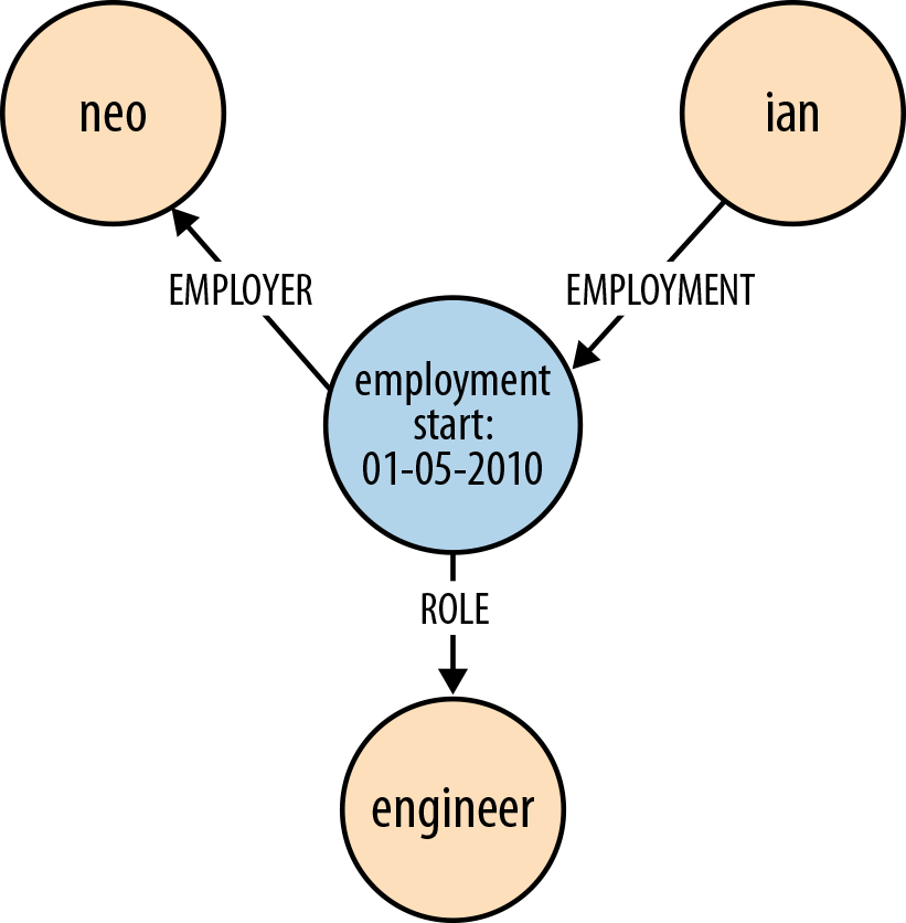
Figure 4-2 shows how the fact of Ian being employed by Neo Technology in the role of engineer can be represented in the graph.

Figure 4-2. Ian was employed as an engineer at Neo Technology

In Cypher, this can be expressed as:

(ian)-[:EMPLOYMENT]->(employment)-[:EMPLOYER]->(neo),
(employment)-[:ROLE]->(engineer)

Performance

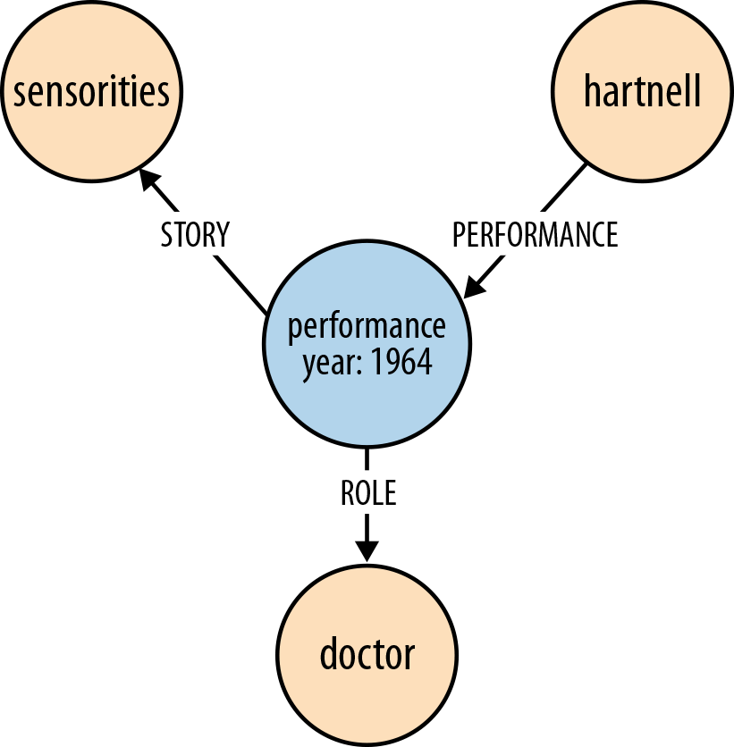
Figure 4-3 shows how the fact of William Hartnell having played the Doctor in the story The Sensorites can be represented in the graph.

Figure 4-3. William Hartnell played the Doctor in the story The Sensorites

In Cypher:

(hartnell)-[:PERFORMANCE]->(performance)-[:ROLE]->(doctor),
(performance)-[:STORY]->(sensorites)

Emailing

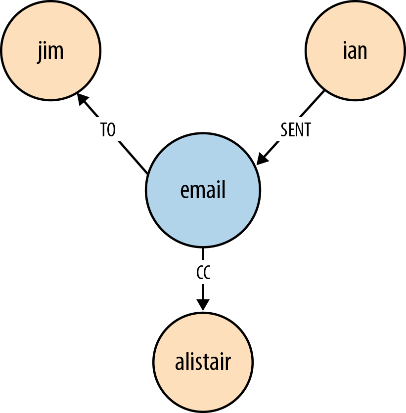
Figure 4-4 shows the act of Ian emailing Jim and copying in Alistair.

Figure 4-4. Ian emailed Jim, and copied in Alistair

In Cypher, this can be expressed as:

(ian)-[:SENT]->(email)-[:TO]->(jim),
(email)-[:CC]->(alistair)

Reviewing

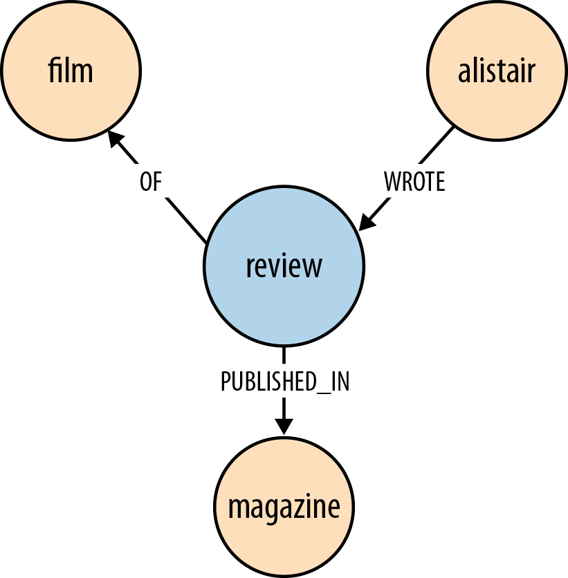
Figure 4-5 shows how the act of Alistair reviewing a film can be represented in the graph.

Figure 4-5. Alistair wrote a review of a film, which was published in a magazine

In Cypher:

(alistair)-[:WROTE]->(review)-[:OF]->(film),
(review)-[:PUBLISHED_IN]->(magazine)

Represent Complex Value Types as Nodes

Value types are things that do not have an identity, and whose equivalence is based solely on their values. Examples include money, address, and SKU. Complex value types are value types with more than one field or property. Address, for example, is a complex value type. Such multiproperty value types are best represented as separate nodes:

START ord=node:orders(orderid={orderId})
MATCH (ord)-[:DELIVERY_ADDRESS]->(address)
RETURN address.first_line, address.zipcode

Time

Time can be modeled in several different ways in the graph. Here we describe two techniques: timeline trees and linked lists.

Timeline trees

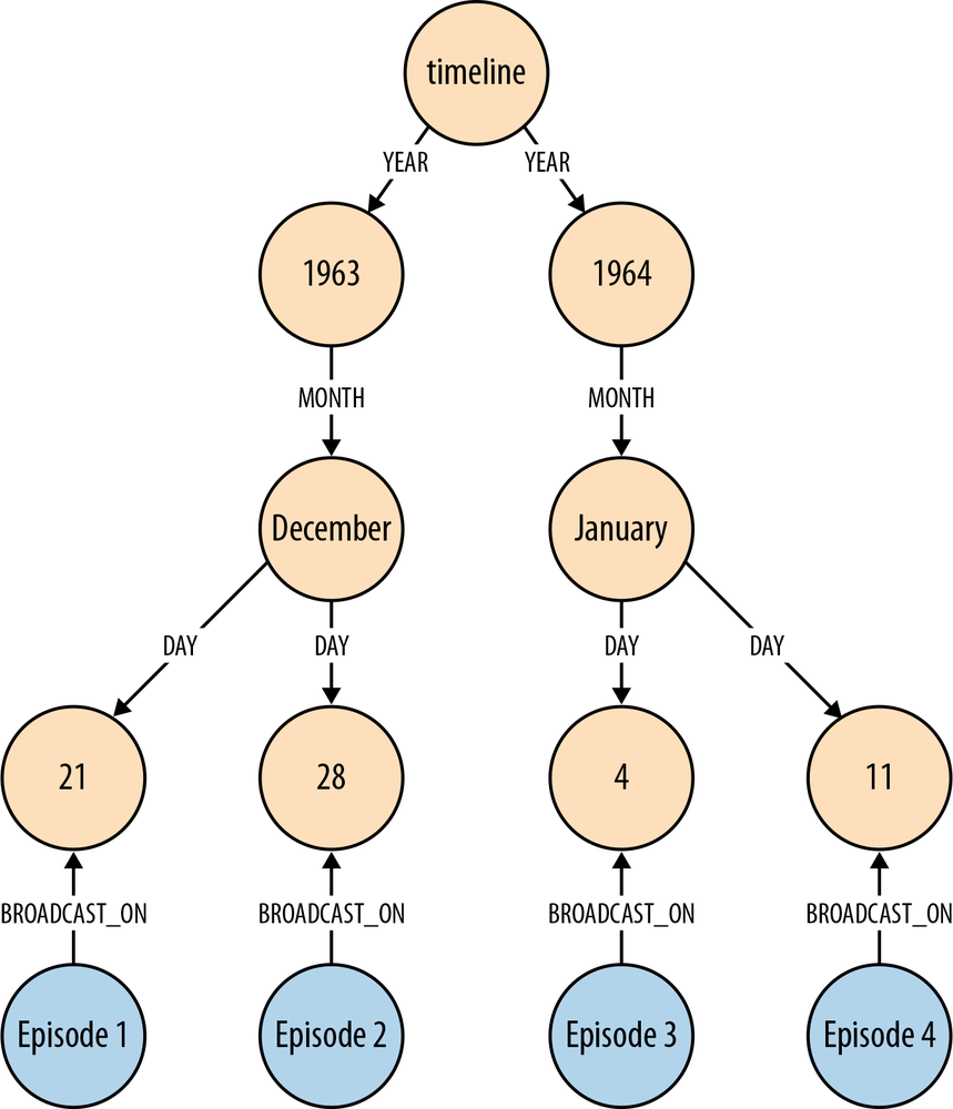
If we need to find all the events that have occurred over a specific period, we can build a timeline tree, as shown in Figure 4-6.

Figure 4-6. A timeline tree showing the broadcast dates for four episodes of a TV program

Each year has its own set of month nodes; each month has its own set of day nodes. We need only insert nodes into the timeline tree as and when they are needed. Assuming the root timeline node has been indexed, or is in some other way discoverable, the following Cypher statement will insert all necessary nodes for a particular event—year, month, day, plus the node representing the event to be attached to the timeline:

START timeline=node:timeline(name={timelineName})
CREATE UNIQUE (timeline)-[:YEAR]->(year{value:{year}, name:{yearName}})
              -[:MONTH]->(month{value:{month}, name:{monthName}})
              -[:DAY]->(day{value:{day}, name:{dayName}})
              <-[:BROADCAST_ON]-(n {newNode})

Querying the calendar for all events between a start date (inclusive) and an end date (exclusive) can be done with the following Cypher:

START timeline=node:timeline(name={timelineName})
MATCH (timeline)-[:YEAR]->(year)-[:MONTH]->(month)-[:DAY]->
      (day)<-[:BROADCAST_ON]-(n)
WHERE ((year.value > {startYear} AND year.value < {endYear})
      OR ({startYear} = {endYear} AND {startMonth} = {endMonth}
          AND year.value = {startYear} AND month.value = {startMonth}
          AND day.value >= {startDay} AND day.value < {endDay})
      OR ({startYear} = {endYear} AND {startMonth} < {endMonth}
          AND year.value = {startYear}
          AND ((month.value = {startMonth} AND day.value >= {startDay})
              OR (month.value > {startMonth} AND month.value < {endMonth})
              OR (month.value = {endMonth} AND day.value < {endDay})))
      OR ({startYear} < {endYear}
          AND year.value = {startYear}
          AND ((month.value > {startMonth})
              OR (month.value = {startMonth} AND day.value >= {startDay})))
      OR ({startYear} < {endYear}
          AND year.value = {endYear}
          AND ((month.value < {endMonth})
              OR (month.value = {endMonth} AND day.value < {endDay}))))
RETURN n

The WHERE clause here, though somewhat verbose, simply filters each match based on the start and end dates supplied to the query.

Linked lists

Many events have temporal relationships to the events that precede and follow them. We can use NEXT and PREVIOUS relationships (or similar) to create linked lists that capture this natural ordering, as shown in Figure 4-7. Linked lists allow for very rapid traversal of time-ordered events.

Figure 4-7. A doubly linked list representing a time-ordered series of events

Versioning

A versioned graph enables us to recover the state of the graph at a particular point in time. Most graph databases don’t support versioning as a first-class concept: it is possible, however, to create a versioning scheme inside the graph model whereby nodes and relationships are timestamped and archived whenever they are modified.^[7] The downside of such versioning schemes is that they leak into any queries written against the graph, adding a layer of complexity to even the simplest query.

Iterative and Incremental Development

We develop the data model feature by feature, user story by user story. This will ensure we identify the relationships our application will use to query the graph. A data model that is developed in line with the iterative and incremental delivery of application features will look quite different from one drawn up using a data model-first approach, but it will be the correct model, motivated throughout by specific needs, and the questions that arise in conjunction with those needs.

Graph databases provide for the smooth evolution of our data model. Migrations and denormalization are rarely an issue. New facts and new compositions become new nodes and relationships, while optimizing for performance-critical access patterns typically involves introducing a direct relationship between two nodes that would otherwise be connected only by way of intermediaries. Unlike the optimization strategies we employ in the relational world, which typically involve denormalizing and thereby compromising a high-fidelity model, this is not an either/or issue: either the detailed, highly normalized structure, or the high performance compromise. With the graph we retain the original high-fidelity graph structure, while at the same time enriching it with new elements that cater to new needs.

We will quickly see how different relationships can sit side-by-side with one another, catering to different needs without distorting the model in favor of any one particular need. Addresses help illustrate the point here. Imagine, for example, that we are developing a retail application. While developing a fulfillment story, we add the ability to dispatch a parcel to a customer’s delivery address, which we find using the following query:

START user=node:users(id={userId})
MATCH (user)-[:DELIVERY_ADDRESS]->(address)
RETURN address

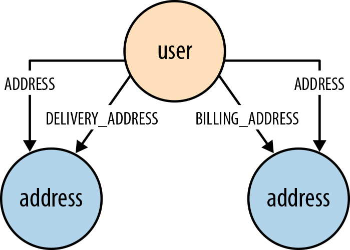
Later on, when adding some billing functionality, we introduce a BILLING_ADDRESS relationship. Later still, we add the ability for customers to manage all their addresses. This last feature requires us to find all addresses—whether delivery, or billing, or some other address. To facilitate this, we introduce a general ADDRESS relationship:

START user=node:users(id={userId})
MATCH (user)-[:ADDRESS]->(address)
RETURN address

By this time, our data model looks something like the one shown in Figure 4-8. DELIVERY_ADDRESS specializes the data on behalf of the application’s fulfillment needs; BILLING_ADDRESS specializes the data on behalf of the application’s billing needs; and ADDRESS specializes the data on behalf of the application’s customer management needs.

Figure 4-8. Different relationships for different application needs

Being able to add new relationships to meet new application needs doesn’t mean we should always do this. We’ll invariably identify opportunities for refactoring the model as we go: there’ll be plenty of times, for example, where renaming an existing relationship will allow it to be used for two different needs. When these opportunities arise, we should take them. If we’re developing our solution in a test-driven manner—described in more detail later in this chapter—we’ll have a sound suite of regression tests in place, enabling us to make substantial changes to the model with confidence.

Application Architecture

In planning a graph database-based solution, there are several architectural decisions to be made. These decisions will vary slightly depending on the database product we’ve chosen; in this section, we’ll describe some of the architectural choices, and the corresponding application architectures, available to us when using Neo4j.

Embedded Versus Server

Most databases today run as a server that is accessed through a client library. Neo4j is somewhat unusual in that it can be run in embedded as well as server mode—in fact, going back nearly ten years, its origins are as an embedded graph database.

Note

An embedded database is not the same as an in-memory database. An embedded instance of Neo4j still makes all data durable on disk. Later, in Testing, we’ll discuss ImpermanentGraphDatabase, which is an in-memory version of Neo4j designed for testing purposes.

Embedded Neo4j

In embedded mode, Neo4j runs in the same process as our application. Embedded Neo4j is ideal for hardware devices, desktop applications, and for incorporating in our own application servers. Some of the advantages of embedded mode include:

Low latency

Because our application speaks directly to the database, there’s no network overhead.

Choice of APIs

We have access to the full range of APIs for creating and querying data: the Core API, traversal framework, and the Cypher query language.

Explicit transactions

Using the Core API, we can control the transactional life cycle, executing an arbitrarily complex sequence of commands against the database in the context of a single transaction. The Java APIs also expose the transaction life cycle, enabling us to plug in custom transaction event handlers that execute additional logic with each transaction.

Named indexes

Embedded mode gives us full control over the creation and management of named indexes. This functionality is also available through the web-based REST interface; it is not, however, available in Cypher.

When running in embedded mode, however, we should bear in mind the following:

JVM only

Neo4j is a JVM-based database. Many of its APIs are, therefore, accessible only from a JVM-based language.

GC behaviors

When running in embedded mode, Neo4j is subject to the garbage collection (GC) behaviors of the host application. Long GC pauses can affect query times. Further, when running an embedded instance as part of an HA cluster, long GC pauses can cause the cluster protocol to trigger a master reelection.

Database life cycle

The application is responsible for controlling the database life cycle, which includes starting it, and closing it safely.

Embedded Neo4j can be clustered for high availability and horizontal read scaling just as the server version. In fact, we can run a mixed cluster of embedded and server instances (clustering is performed at the database level, rather than the server level). This is common in enterprise integration scenarios, where regular updates from other systems are executed against an embedded instance, and then replicated out to server instances.

Server mode

Running Neo4j in server mode is the most common means of deploying the database today. At the heart of each server is an embedded instance of Neo4j. Some of the benefits of server mode include:

REST API

The server exposes a rich REST API that allows clients to send JSON-formatted requests over HTTP. Responses comprise JSON-formatted documents enriched with hypermedia links that advertise additional features of the dataset.

Platform independence

Because access is by way of JSON-formatted documents sent over HTTP, a Neo4j server can be accessed by a client running on practically any platform. All that’s needed is an HTTP client library.^[8]

Scaling independence

With Neo4j running in server mode, we can scale our database cluster independently of our application server cluster.

Isolation from application GC behaviors

In server mode, Neo4j is protected from any untoward GC behaviors triggered by the rest of the application. Of course, Neo4j still produces some garbage, but its impact on the garbage collector has been carefully monitored and tuned during development to mitigate any significant side effects. However, because server extensions enable us to run arbitrary Java code inside the server (see ), the use of server extensions may impact the server’s GC behavior.

When using Neo4j in server mode, we should bear in mind the following:

Network overhead

There is some communication overhead to each HTTP request, though it’s fairly minimal. After the first client request, the TCP connection remains open until closed by the client.

Per-request transactions

Each client request is executed in the context of a separate transaction, though there is some support in the REST API for batch operations. For more complex, multistep operations requiring a single transactional context, we should consider using a server extension (see ).

Access to Neo4j server is typically by way of its REST API, as discussed previously. The REST API comprises JSON-formatted documents over HTTP. Using the REST API we can submit Cypher queries, configure named indexes, and execute several of the built-in graph algorithms. We can also submit JSON-formatted traversal descriptions, and perform batch operations. For the majority of use cases the REST API is sufficient; however, if we need to do something we cannot currently accomplish using the REST API, we should consider developing a server extension.

Server extensions

Server extensions enable us to run Java code inside the server. Using server extensions, we can extend the REST API, or replace it entirely.

Extensions take the form of JAX-RS annotated classes. JAX-RS is a Java API for building RESTful resources. Using JAX-RS annotations, we decorate each extension class to indicate to the server which HTTP requests it handles. Additional annotations control request and response formats, HTTP headers, and the formatting of URI templates.

Here’s an implementation of a simple server extension that allows a client to request the distance between two members of a social network:

@Path("/distance")
public class SocialNetworkExtension
{
    private final ExecutionEngine executionEngine;

    public SocialNetworkExtension( @Context GraphDatabaseService db )
    {
        this.executionEngine = new ExecutionEngine( db );
    }

    @GET
    @Produces("text/plain")
    @Path("/{name1}/{name2}")
    public String getDistance  ( @PathParam("name1") String name1,
                                 @PathParam("name2") String name2 )
    {
        String query = "START first=node:user(name={name1}),\n" +
                "second=node:user(name={name2})\n" +
                "MATCH p=shortestPath(first-[*..4]-second)\n" +
                "RETURN length(p) AS depth";

        Map<String, Object> params = new HashMap<String, Object>();
        params.put( "name1", name1 );
        params.put( "name2", name2 );

        ExecutionResult result = executionEngine.execute( query, params );

        return String.valueOf( result.columnAs( "depth" ).next() );
    }
}

Of particular interest here are the various annotations:

• @Path("/distance") specifies that this extension will respond to requests directed to relative URIs beginning /distance.
• The @Path("/{name1}/{name2}") annotation on getDistance() further qualifies the URI template associated with this extension. The fragment here is concatenated with /distance to produce /distance/{name1}/{name2}, where {name1} and {name2} are placeholders for any characters occurring between the forward slashes. Later on, in Testing server extensions, we’ll register this extension under the /socnet relative URI. At that point, these several different parts of the path ensure that HTTP requests directed to a relative URI beginning /socnet/distance/{name1}/{name2} (for example, http://<server>/socnet/distance/Ben/Mike) will be dispatched to an instance of this extension.
• @GET specifies that getDistance() should be invoked only if the request is an HTTP GET. @Produces indicates that the response entity body will be formatted as text/plain.
• The two @PathParam annotations prefacing the parameters to getDistance() serve to map the contents of the {name1} and {name2} path placeholders to the method’s name1 and name2 parameters. Given the URI http://<server>/socnet/distance/Ben/Mike, getDistance() will be invoked with Ben for name1 and Mike for name2.
• The @Context annotation in the constructor causes this extension to be handed a reference to the embedded graph database inside the server. The server infrastructure takes care of creating an extension and injecting it with a graph database instance, but the very presence of the GraphDatabaseService parameter here makes this extension exceedingly testable. As we’ll see later, in , we can unit test extensions without having to run them inside a server.

Server extensions can be powerful elements in our application architecture. Their chief benefits include:

Complex transactions

Extensions enable us to execute an arbitrarily complex sequence of operations in the context of a single transaction.

Choice of APIs

Each extension is injected with a reference to the embedded graph database at the heart of the server. This gives us access to the full range of APIs—Core API, traversal framework, graph algorithm package, and Cypher—for developing our extension’s behavior.

Encapsulation

Because each extension is hidden behind a RESTful interface, we can improve and modify its implementation over time.

Response formats

We control the response: both the representation format and the HTTP headers. This enables us to create response messages whose contents employ terminology from our domain, rather than the graph-based terminology of the standard REST API (users, products, and orders for example, rather than nodes, relationships, and properties). Further, in controlling the HTTP headers attached to the response, we can leverage the HTTP protocol for things such as caching and conditional requests.

When considering using server extensions, we should bear in mind the following points:

JVM only

As with developing against embedded Neo4j, we’ll have to use a JVM-based language.

GC behaviors

We can do arbitrarily complex (and dangerous) things inside a server extension. We need to monitor garbage collection behaviors to ensure we don’t introduce any untoward side effects.

Clustering

As we discuss in more detail later, in Availability, Neo4j clusters for high availability and horizontal read scaling using master-slave replication. In this section we discuss some of the strategies to consider when using clustered Neo4j.

Replication

Although all writes to a cluster are coordinated through the master, Neo4j does allow writing through slaves, but even then, the slave that’s being written to syncs with the master before returning to the client. Because of the additional network traffic and coordination protocol, writing through slaves can be an order of magnitude slower than writing directly to the master. The only reasons for writing through slaves are to increase the durability guarantees of each write (the write is made durable on two instances, rather than one) and to ensure we can read our own writes when employing cache sharding (see Cache sharding and Read your own writes later in this chapter). Because newer versions of Neo4j enable us to specify that writes to the master must be replicated out to one or more slaves, thereby increasing the durability guarantees of writes to the master, the case for writing through slaves is now less compelling. Today it is recommended that all writes be directed to the master, and then replicated to slaves using the ha.tx_push_factor and ha.tx_push_strategy configuration settings.

Buffer writes using queues

In high write load scenarios, we can use queues to buffer writes and regulate load. With this strategy, writes to the cluster are buffered in a queue; a worker then polls the queue and executes batches of writes against the database. Not only does this regulate write traffic, but it reduces contention, and enables us to pause write operations without refusing client requests during maintenance periods.

Global clusters

For applications catering to a global audience, it is possible to install a multiregion cluster in multiple data centers and on cloud platforms such as Amazon Web Services (AWS). A multiregion cluster enables us to service reads from the portion of the cluster geographically closest to the client. In these situations, however, the latency introduced by the physical separation of the regions can sometimes disrupt the coordination protocol; it is, therefore, often desirable to restrict master reelection to a single region. To achieve this, we create slave-only databases for the instances we don’t want to participate in master reelection; we do this by including the ha.slave_coordinator_update_mode=none configuration parameter in an instance’s configuration.

Load Balancing

When using a clustered graph database, we should consider load balancing traffic across the cluster to help maximize throughput and reduce latency. Neo4j doesn’t include a native load balancer, relying instead on the load-balancing capabilities of the network infrastructure.

Separate read traffic from write traffic

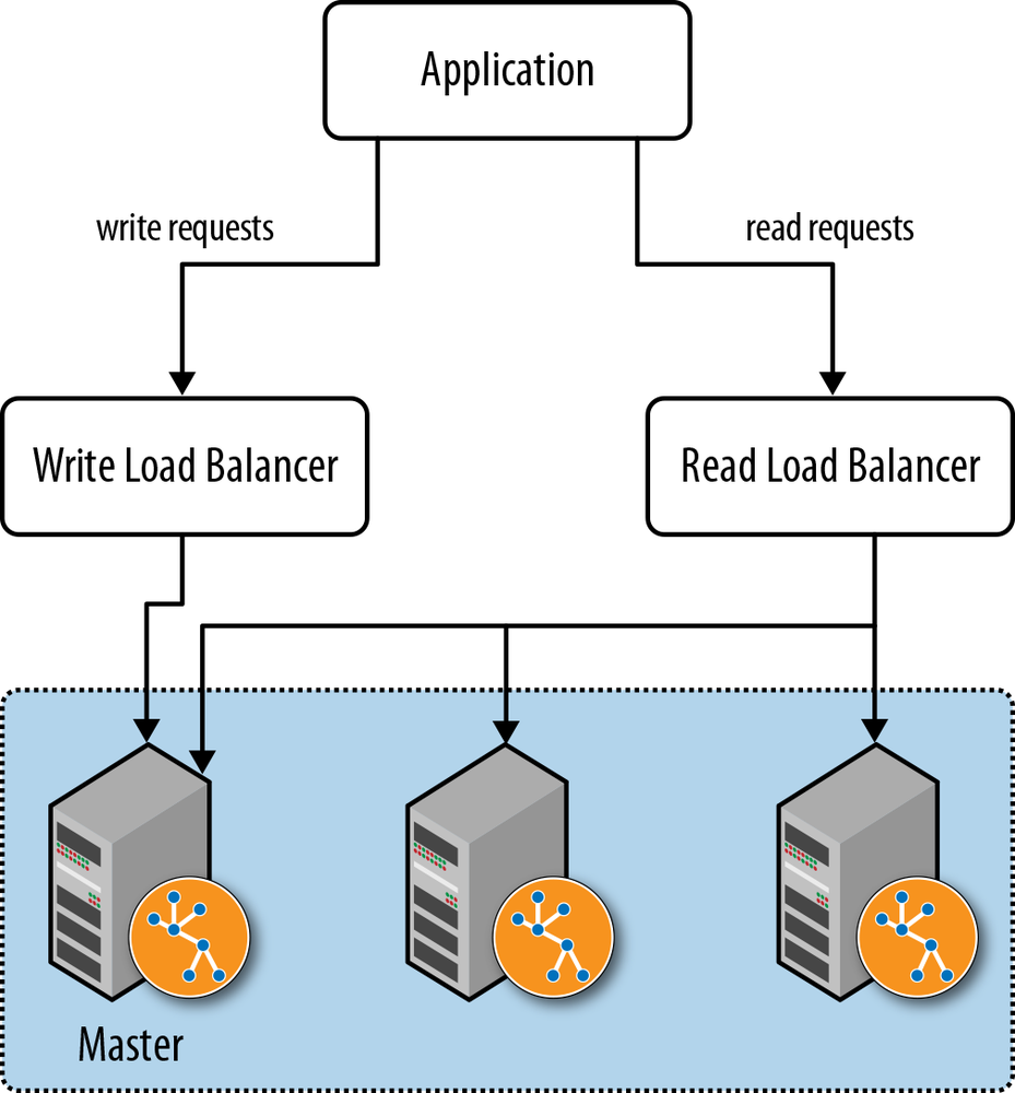
Given the recommendation to direct the majority of write traffic to the master, we should consider clearly separating read requests from write requests. We should configure our load balancer to direct write traffic to the master, while balancing the read traffic across the entire cluster.

In a web-based application, the HTTP method is often sufficient to distinguish a request with a significant side effect—a write—from one that has no significant side effect on the server: POST, PUT, and DELETE can modify server-side resources, whereas GET is side-effect free.

When using server extensions, it’s important to distinguish read and write operations using @GET and @POST annotations. If our application depends solely on server extensions, this will suffice to separate the two. If we’re using the REST API to submit Cypher queries to the database, however, the situation is not so straightforward. The REST API uses POST as a general “process this” semantic for requests whose contents can include Cypher statements that modify the database. To separate read and write requests in this scenario, we introduce a pair of load balancers: a write load balancer that always directs requests to the master, and a read load balancer that balances requests across the entire cluster. In our application logic, where we know whether the operation is a read or a write, we will then have to decide which of the two addresses we should use for any particular request, as illustrated in Figure 4-9.

When running in server mode, Neo4j exposes a URI that indicates whether that instance is currently the master, and if it isn’t, which is. Load balancers can poll this URI at intervals to determine where to route traffic.

Cache sharding

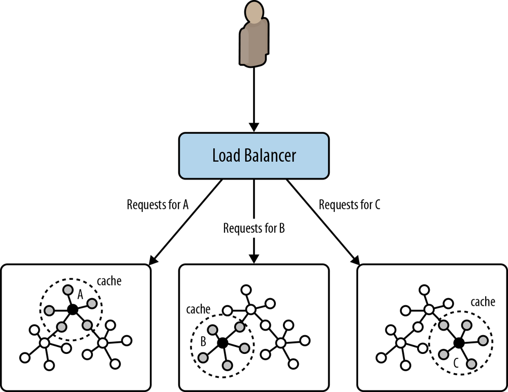
Queries run fastest when the portions of the graph needed to satisfy them reside in main memory (that is, in the filesystem cache and the object cache). A single graph database instance today can hold many billions of nodes, relationships, and properties, meaning that some graphs will be just too big to fit into main memory. Partitioning or sharding a graph is a difficult problem to solve (see The Holy Grail of Graph Scalability). How, then, can we provide for high-performance queries over a very large graph?

One solution is to use a technique called cache sharding (Figure 4-10), which consists of routing each request to a database instance in an HA cluster where the portion of the graph necessary to satisfy that request is likely already in main memory (remember: every instance in the cluster will contain a full copy of the data). If the majority of an application’s queries are graph-local queries, meaning they start from one or more specific points in the graph, and traverse the surrounding subgraphs, then a mechanism that consistently routes queries beginning from the same set of start points to the same database instance will increase the likelihood of each query hitting a warm cache.

Figure 4-9. Using read/write load balancers to direct requests to a cluster

The strategy used to implement consistent routing will vary by domain. Sometimes it’s good enough to have sticky sessions; other times we’ll want to route based on the characteristics of the dataset. The simplest strategy is to have the instance that first serves requests for a particular user thereafter serve subsequent requests for that user. Other domain-specific approaches will also work. For example, in a geographical data system we can route requests about particular locations to specific database instances that have been warmed for that location. Both strategies increase the likelihood of the required nodes and relationships already being cached in main memory, where they can be quickly accessed and processed.

Figure 4-10. Cache sharding

Read your own writes

Occasionally we may need to read our own writes—typically when the application applies an end-user change, and needs on the next request to reflect the effect of this change back to the user. Whereas writes to the master are immediately consistent, the cluster as a whole is eventually consistent. How can we ensure that a write directed to the master is reflected in the next load-balanced read request? One solution is to use the same consistent routing technique used in cache sharding to direct the write to the slave that will be used to service the subsequent read. This assumes that the write and the read can be consistently routed based on some domain criteria in each request.

This is one of the few occasions where it makes sense to write through a slave. But remember: writing through a slave can be an order of magnitude slower than writing directly to the master. We should use this technique sparingly. If a high proportion of our writes require us to read our own write, this technique will significantly impact throughput and latency.

Testing

Testing is a fundamental part of the application development process—not only as a means of verifying that a query or application feature behaves correctly, but also as a way of designing and documenting our application and its data model. Throughout this section we emphasize that testing is an everyday activity; by developing our graph database solution in a test-driven manner, we provide for the rapid evolution of our system, and its continued responsiveness to new business needs.

Test-Driven Data Model Development

In discussing data modeling, we’ve stressed that our graph model should reflect the kinds of queries we want to run against it. By developing our data model in a test-driven fashion we document our understanding of our domain, and validate that our queries behave correctly.

With test-driven data modeling, we write unit tests based on small, representative example graphs drawn from our domain. These example graphs contain just enough data to communicate a particular feature of the domain; in many cases, they might only comprise 10 or so nodes, plus the relationships that connect them. We use these examples to describe what is normal for the domain, and also what is exceptional. As we discover anomalies and corner cases in our real data, we write a test that reproduces what we’ve discovered.

The example graphs we create for each test comprise the setup or context for that test. Within this context we exercise a query, and assert that the query behaves as expected. Because we control the context, we, as the author of the test, know what results to expect.

Tests can act like documentation. By reading the tests, developers gain an understanding of the problems and needs the application is intended to address, and the ways in which the authors have gone about addressing them. With this is mind, it’s best to use each test to test just one aspect of our domain. It’s far easier to read lots of small tests, each of which communicates a discrete feature of our data in a clear, simple, and concise fashion, than it is to reverse engineer a complex domain from a single large and unwieldy test. In many cases, we’ll find a particular query being exercised by several tests, some of which demonstrate the happy path through our domain, others of which exercise it in the context of some exceptional structure or set of values.^[9]

Over time, we’ll build up a suite of tests that can act as a powerful regression test mechanism. As our application evolves, and we add new sources of data, or change the model to meet new needs, our regression test suite will continue to assert that existing features continue to behave as they should. Evolutionary architectures, and the incremental and iterative software development techniques that support them, depend upon a bedrock of asserted behavior. The unit-testing approach to data model development described here enables developers to respond to new business needs with very little risk of undermining or breaking what has come before, confident in the continued quality of the solution.

Example: A test-driven social network data model

In this example we’re going to demonstrate developing a very simple Cypher query for a social network. Given the names of a couple of members of the network, our query determines the distance between them.

First we create a small graph that is representative of our domain. Using Cypher, we create a network comprising ten nodes and eight relationships:

public GraphDatabaseService createDatabase()
{
    // Create nodes
    String cypher = "CREATE\n" +
            "(ben {name:'Ben'}),\n" +
            "(arnold {name:'Arnold'}),\n" +
            "(charlie {name:'Charlie'}),\n" +
            "(gordon {name:'Gordon'}),\n" +
            "(lucy {name:'Lucy'}),\n" +
            "(emily {name:'Emily'}),\n" +
            "(sarah {name:'Sarah'}),\n" +
            "(kate {name:'Kate'}),\n" +
            "(mike {name:'Mike'}),\n" +
            "(paula {name:'Paula'}),\n" +
            "ben-[:FRIEND]->charlie,\n" +
            "charlie-[:FRIEND]->lucy,\n" +
            "lucy-[:FRIEND]->sarah,\n" +
            "sarah-[:FRIEND]->mike,\n" +
            "arnold-[:FRIEND]->gordon,\n" +
            "gordon-[:FRIEND]->emily,\n" +
            "emily-[:FRIEND]->kate,\n" +
            "kate-[:FRIEND]->paula";

    GraphDatabaseService db =
                new TestGraphDatabaseFactory().newImpermanentDatabase();

    ExecutionEngine engine = new ExecutionEngine( db );
    engine.execute( cypher );

    // Index all nodes in "user" index
    Transaction tx = db.beginTx();
    try
    {
        Iterable<Node> allNodes =
                GlobalGraphOperations.at( db ).getAllNodes();
        for ( Node node : allNodes )
        {
            if ( node.hasProperty( "name" ) )
            {
                db.index().forNodes( "user" )
                        .add( node, "name", node.getProperty( "name" ) );
            }
        }
        tx.success();
    }
    finally
    {
        tx.finish();
    }

    return db;
}

There are two things of interest in createDatabase(). The first is the use of ImpermanentGraphDatabase, which is a lightweight, in-memory version of Neo4j designed specifically for unit testing. By using ImpermanentGraphDatabase, we avoid having to clear up store files on disk after each test. The class can be found in the Neo4j kernel test jar, which can be obtained with the following dependency reference:

<dependency>
    <groupId>org.neo4j</groupId>
    <artifactId>neo4j-kernel</artifactId>
    <version>${project.version}</version>
    <type>test-jar</type>
    <scope>test</scope>
</dependency>

Warning

ImpermanentGraphDatabase should only be used in unit tests. It is not a production-ready, in-memory version of Neo4j.

The second thing of interest in createDatabase() is the code for adding nodes to a named index. Cypher doesn’t add the newly created nodes to an index, so for now, we have to do this manually by iterating all the nodes in the sample graph, adding any with a name property to the users named index.

Having created a sample graph, we can now write our first test. Here’s the test fixture for testing our social network data model and its queries:

public class SocialNetworkTest
{
    private static GraphDatabaseService db;
    private static SocialNetworkQueries queries;

    @BeforeClass
    public static void init()
    {
        db = createDatabase();
        queries = new SocialNetworkQueries( db );
    }

    @AfterClass
    public static void shutdown()
    {
        db.shutdown();
    }

    @Test
    public void shouldReturnShortestPathBetweenTwoFriends() throws Exception
    {
        // when
        ExecutionResult results = queries.distance( "Ben", "Mike" );

        // then
        assertTrue( results.iterator().hasNext() );
        assertEquals( 4, results.iterator().next().get( "distance" ) );
    }

    // more tests
}

This test fixture includes an initialization method, annotated with @BeforeClass, which executes before any tests start. Here we call createDatabase() to create an instance of the sample graph, and an instance of SocialNetworkQueries, which houses the queries under development.

Our first test, shouldReturnShortestPathBetweenTwoFriends(), tests that the query under development can find a path between any two members of the network—in this case, Ben and Mike. Given the contents of the sample graph, we know that Ben and Mike are connected, but only remotely, at a distance of 4. The test, therefore, asserts that the query returns a nonempty result containing a distance value of 4.

Having written the test, we now start developing our first query. Here’s the implementation of SocialNetworkQueries:

public class SocialNetworkQueries
{
    private final ExecutionEngine executionEngine;

    public SocialNetworkQueries( GraphDatabaseService db )
    {
        this.executionEngine = new ExecutionEngine( db );
    }

    public ExecutionResult distance( String firstUser, String secondUser )
    {
        String query = "START first=node:user({firstUserQuery}),\n" +
                "second=node:user({secondUserQuery})\n" +
                "MATCH p=shortestPath(first-[*..4]-second)\n" +
                "RETURN length(p) AS distance";

        Map<String, Object> params = new HashMap<String, Object>();
        params.put( "firstUserQuery", "name:" + firstUser );
        params.put( "secondUserQuery", "name:" + secondUser );

        return executionEngine.execute( query, params );
    }

    // More queries
}

In the constructor for SocialNetworkQueries we create a Cypher ExecutionEngine, passing in the supplied database instance. We store the execution engine in a member variable, which allows it to be reused over and again throughout the lifetime of the queries instance. The query itself we implement in the distance() method. Here we create a Cypher statement, initialize a map containing the query parameters, and execute the statement using the execution engine.

If shouldReturnShortestPathBetweenTwoFriends() passes (it does), we then go on to test additional scenarios. What happens, for example, if two members of the network are separated by more than four connections? We write up the scenario and what we expect the query to do in another test:

@Test
public void shouldReturnNoResultsWhenNoPathUnderAtDistance4OrLess()
    throws Exception
{
    // when
    ExecutionResult results = queries.distance( "Ben", "Arnold" );

    // then
    assertFalse( results.iterator().hasNext() );
}

In this instance, this second test passes without us having to modify the underlying Cypher query. In many cases, however, a new test will force us to modify a query’s implementation. When that happens, we modify the query to make the new test pass, and then run all the tests in the fixture. A failing test anywhere in the fixture indicates we’ve broken some existing functionality. We continue to modify the query until all tests are green once again.

Testing server extensions

Server extensions can be developed in a test-driven manner just as easily as embedded Neo4j. Using the simple server extension described earlier, here’s how we test it:

@Test
public void extensionShouldReturnDistance() throws Exception
{
    // given
    SocialNetworkExtension extension = new SocialNetworkExtension( db );

    // when
    String distance = extension.getDistance( "Ben", "Mike" );

    // then
    assertEquals( "4", distance );
}

Because the extension’s constructor accepts a GraphDatabaseService instance, we can inject a test instance (an ImpermanentGraphDatabase instance), and then call its methods as per any other object.

If, however, we wanted to test the extension running inside a server, we have a little more setup to do:

public class SocialNetworkExtensionTest
{
    private static CommunityNeoServer server;

    @BeforeClass
    public static void init() throws IOException
    {
        server = ServerBuilder.server()
                .withThirdPartyJaxRsPackage(
                        "org.neo4j.graphdatabases.queries.server",
                        "/socnet" )
                .build();
        server.start();
        populateDatabase( server.getDatabase().getGraph() );
    }

    @AfterClass
    public static void teardown()
    {
        server.stop();
    }

    @Test
    public void serverShouldReturnDistance() throws Exception
    {
        ClientConfig config = new DefaultClientConfig();
        Client client = Client.create( config );

        WebResource resource = client
                .resource( "http://localhost:7474/socnet/distance/Ben/Mike" );
        ClientResponse response = resource
                .accept( MediaType.TEXT_PLAIN )
                .get( ClientResponse.class );

        assertEquals( 200, response.getStatus() );
        assertEquals( "text/plain",
                response.getHeaders().get( "Content-Type" ).get( 0 ) );
        assertEquals( "4", response.getEntity( String.class ) );
    }

    // Populate graph

}

Here we’re using an instance of CommunityNeoServer to host the extension. We create the server and populate its database in the test fixture’s init() method using a ServerBuilder, which is a helper class from Neo4j’s server test jar. This builder enables us to register the extension package, and associate it with a relative URI space (in this case, everything below /socnet). Once init() has completed, we have a server instance up and running and listening on port 7474.

In the test itself, serverShouldReturnDistance(), we access this server using an HTTP client from the Jersey client library. The client issues an HTTP GET request for the resource at http://localhost:7474/socnet/distance/Ben/Mike. (At the server end, this request is dispatched to an instance of SocialNetworkExtension.) When the client receives a response, the test asserts that the HTTP status code, content-type, and content of the response body are correct.

Performance Testing

The test-driven approach that we’ve described so far communicates context and domain understanding, and tests for correctness. It does not, however, test for performance. What works fast against a small, 20-node sample graph may not work so well when confronted with a much larger graph. Therefore, to accompany our unit tests, we should consider writing a suite of query performance tests. On top of that, we should also invest in some thorough application performance testing early in our application’s development life cycle.

Query performance tests

Query performance tests are not the same as full-blown application performance tests. All we’re interested in at this stage is whether a particular query performs well when run against a graph that is proportionate to the kind of graph we expect to encounter in production. Ideally, these tests are developed side-by-side with our unit tests. There’s nothing worse than investing a lot of time in perfecting a query, only to discover it is not fit for production-sized data.

When creating query performance tests, bear in mind the following guidelines:

• Create a suite of performance tests that exercise the queries developed through our unit testing. Record the performance figures so that we can see the relative effects of tweaking a query, modifying the heap size, or upgrading from one version of a graph database to another.
• Run these tests often, so that we quickly become aware of any deterioration in performance. We might consider incorporating these tests into a continuous delivery build pipeline, failing the build if the test results exceed a certain value.
• Run these tests in-process on a single thread. There’s no need to simulate multiple clients at this stage: if the performance is poor for a single client, it’s unlikely to improve for multiple clients. Even though they are not, strictly speaking, unit tests, we can drive them using the same unit testing framework we use to develop our unit tests.
• Run each query many times, picking starting nodes at random each time, so that we can see the effect of starting from a cold cache, which is then gradually warmed as multiple queries execute.

Application performance tests

Application performance tests, as distinct from query performance tests, test the performance of the entire application under representative production usage scenarios.

As with query performance tests, we recommend that this kind of performance testing is done as part of everyday development, side-by-side with the development of application features, rather than as a distinct project phase.^[10] To facilitate application performance testing early in the project life cycle, it is often necessary to develop a “walking skeleton,” an end-to-end slice through the entire system, which can be accessed and exercised by performance test clients. By developing a walking skeleton, we not only provide for performance testing, but we also establish the architectural context for the graph database part of our solution. This enables us to verify our application architecture, and identify layers and abstractions that allow for discrete testing of individual components.

Performance tests serve two purposes: they demonstrate how the system will perform when used in production, and they drive out the operational affordances that make it easier to diagnose performance issues, incorrect behavior, and bugs. What we learn in creating and maintaining a performance test environment will prove invaluable when it comes to deploying and operating the system for real.

When drawing up the criteria for a performance test, we recommend specifying percentiles rather than averages. Never assume a normal distribution of response times: the real world doesn’t work like that. For some applications we may want to ensure that all requests return within a certain time period. In rare circumstances it may be important for the very first request to be as quick as when the caches have been warmed. But in the majority of cases, we will want to ensure the majority of requests return within a certain time period; that, say, 98% of requests are satisfied in under 200 ms. It is important to keep a record of subsequent test runs so that we can compare performance figures over time, and thereby quickly identify slowdowns and anomalous behavior.

As with unit tests and query performance tests, application performance tests prove most valuable when employed in an automated delivery pipeline, where successive builds of the application are automatically deployed to a testing environment, the tests executed, and the results automatically analyzed. Log files and test results should be stored for later retrieval, analysis, and comparison. Regressions and failures should fail the build, prompting developers to address the issues in a timely manner. One of the big advantages of conducting performance testing over the course of an application’s development life cycle, rather than at the end, is that failures and regressions can very often be tied back to a recent piece of development; this enables us to diagnose, pinpoint, and remedy issues rapidly and succinctly.

For generating load, we’ll need a load-generating agent. For web applications, there are several open source stress and load testing tools available, including Grinder, JMeter, and Gatling.^[11] When testing load-balanced web applications, we should ensure our test clients are distributed across different IP addresses so that requests are balanced across the cluster.

Testing with representative data

For both query performance testing and application performance testing we will need a dataset that is representative of the data we will encounter in production. It will, therefore, be necessary to create or otherwise source such a dataset. In some cases we can obtain a dataset from a third party, or adapt an existing dataset that we own, but unless these datasets are already in the form of a graph, we will have to write some custom export-import code.

In many cases, however, we’re starting from scratch. If this is the case, we must dedicate some time to creating a dataset builder. As with the rest of the software development life cycle, this is best done in an iterative and incremental fashion. Whenever we introduce a new element into our domain’s data model, as documented and tested in our unit tests, we add the corresponding element to our performance dataset builder. That way, our performance tests will come as close to real-world usage as our current understanding of the domain allows.

When creating a representative dataset, we try to reproduce any domain invariants we have identified: the minimum, maximum, and average number of relationships per node, the spread of different relationship types, property value ranges, and so on. Of course, it’s not always possible to know these things upfront, and often we’ll find ourselves working with rough estimates until such point as production data is available to verify our assumptions.

Although ideally we would always test with a production-sized dataset, it is often not possible or desirable to reproduce extremely large volumes of data in a test environment. In such cases, we should at least ensure that we build a representative dataset whose size exceeds the capacity of the object cache. That way, we’ll be able to observe the effect of cache evictions, and querying for portions of the graph not currently held in main memory.

Representative datasets also help with capacity planning. Whether we create a full-sized dataset, or a scaled-down sample of what we expect the production graph to be, our representative dataset will give us some useful figures for estimating the size of the production data on disk. These figures then help us plan how much memory to allocate to the filesystem cache and the Java virtual machine (JVM) heap (see Capacity Planning for more details).

In the following example we’re using a dataset builder called Neode to build a sample social network:^[12]

private void createSampleDataset( GraphDatabaseService db )
{
    DatasetManager dsm = new DatasetManager( db, new Log()
    {
        @Override
        public void write( String value )
        {
            System.out.println(value);
        }
    } );

    // User node specification
    NodeSpecification userSpec =
            dsm.nodeSpecification( "user",
                                   indexableProperty( "name" ) );

    // FRIEND relationship specification
    RelationshipSpecification friend =
            dsm.relationshipSpecification( "FRIEND" );

    Dataset dataset =
            dsm.newDataset( "Social network example" );

    // Create user nodes
    NodeCollection users =
            userSpec.create( 1000000 )
                    .update( dataset );


    // Relate users to each other
    users.createRelationshipsTo(
            getExisting( users )
                    .numberOfTargetNodes( minMax( 50, 100 ) )
                    .relationship( friend )
                    .relationshipConstraints( BOTH_DIRECTIONS ) )
            .updateNoReturn( dataset );

    dataset.end();
}

Neode uses node and relationship specifications to describe the nodes and relationships in the graph, together with their properties and permitted property values. Neode then provides a fluent interface for creating and relating nodes.

Capacity Planning

At some point in our application’s development life cycle we’ll want to start planning for production deployment. In many cases, an organization’s project management gating processes mean a project cannot get underway without some understanding of the production needs of the application. Capacity planning is essential both for budgeting purposes and for ensuring there is sufficient lead time for procuring hardware and reserving production resources.

In this section we describe some of the techniques we can use for hardware sizing and capacity planning. Our ability to estimate our production needs depends on a number of factors: the more data we have regarding representative graph sizes, query performance, and the number of expected users and their behaviors, the better our ability to estimate our hardware needs. We can gain much of this information by applying the techniques described in Testing early in our application development life cycle. In addition, we should understand the cost/performance trade-offs available to us in the context of our business needs.

Optimization Criteria

As we plan our production environment we will be faced with a number of optimization choices. Which we favor will depend upon our business needs:

Cost

We can optimize for cost by installing the minimum hardware necessary to get the job done.

Performance

We can optimize for performance by procuring the fastest solution (subject to budgetary constraints).

Redundancy

We can optimize for redundancy and availability by ensuring the database cluster is big enough to survive a certain number of machine failures (i.e., to survive two machines failing, we will need a cluster comprising five instances).

Load

With a replicated graph database solution, we can optimize for load by scaling horizontally (for read load), and vertically (for write load).

Performance

Redundancy and load can be costed in terms of the number of machines necessary to ensure availability (five machines to provide continued availability in the face of two machines failing, for example) and scalability (one machine per some number of concurrent requests, as per the calculations in Load). But what about performance? How can we cost performance?

Calculating the cost of graph database performance

In order to understand the cost implications of optimizing for performance, we need to understand the performance characteristics of the database stack. As we describe in more detail later in Native Graph Storage, a graph database uses disk for durable storage, and main memory for caching portions of the graph. In Neo4j, the caching parts of main memory are further divided between the filesystem cache (which is typically managed by the operating system) and the object cache. The filesystem cache is a portion of off-heap RAM into which files on disk are read and cached before being served to the application. The object cache is an on-heap cache that stores object instances of nodes, relationships, and properties.

Spinning disk is by far the slowest part of the database stack. Queries that have to reach all the way down to spinning disk will be orders of magnitude slower than queries that touch only the object cache. Disk access can be improved by using solid-state drives (SSDs) in place of spinning disks, providing an approximate 20 times increase in performance, or by using enterprise flash hardware, which can reduce latencies even further.

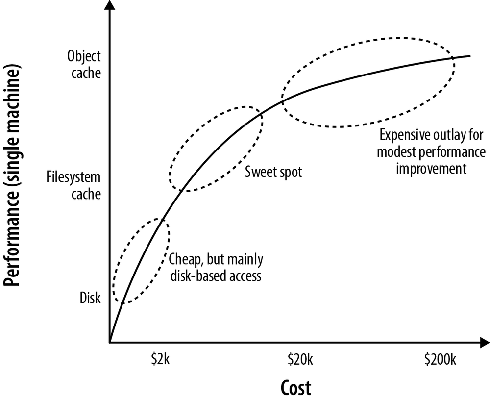
Spinning disks and SDDs are cheap, but not very fast. Far more significant performance benefits accrue when the database has to deal only with the caching layers. The filesystem cache offers up to 500 times the performance of spinning disk, whereas the object cache can be up to 5,000 times faster.

For comparative purposes, graph database performance can be expressed as a function of the percentage of data available at each level of the object cache-filesystem cache-disk hierarchy:

(% graph in object cache x 5000) * (% graph in filesystem cache * 500) * 20 (if using SSDs)

An application in which 100% of the graph is available in the object cache (as well as in the filesystem cache, and on disk) will be more performant than one in which 100% is available on disk, but only 80% in the filesystem cache and 20% in the object cache.

Performance optimization options

There are, then, three areas in which we can optimize for performance:

• Increase the object cache (from 2 GB, all the way up to 200 GB or more in exceptional circumstances)
• Increase the percentage of the store mapped into the filesystem cache
• Invest in faster disks: SSDs or enterprise flash hardware

The first two options here require adding more RAM. In costing the allocation of RAM, however, there are a couple of things to bear in mind. First, whereas the size of the store files in the filesystem cache map one-to-one with the size on disk, graph objects in the object cache can be up to 10 times bigger than their on-disk representations. Allocating RAM to the object cache is, therefore, far more expensive per graph element than allocating it to the filesystem cache. The second point to bear in mind relates to the location of the object cache. If our graph database uses an on-heap cache, as does Neo4j, then increasing the size of the cache requires allocating more heap. Most modern JVMs do not cope well with heaps much larger than 8 GB. Once we start growing the heap beyond this size, garbage collection can impact the performance of our application.^[13]

As Figure 4-11 shows, the sweet spot for any cost versus performance trade-off lies around the point where we can map our store files in their entirety into RAM, while allowing for a healthy, but modestly sized object cache. Heaps of between 4 and 8 GB are not uncommon, though in many cases, a smaller heap can actually improve performance (by mitigating expensive GC behaviors).

Calculating how much RAM to allocate to the heap and the filesystem cache depends on our knowing the projected size of our graph. Building a representative dataset early in our application’s development life cycle will furnish us with some of the data we need to make our calculations. If we cannot fit the entire graph into main memory (that is, at a minimum, into the filesystem cache), we should consider cache sharding (see Cache sharding).

Note

The Neo4j documentation includes details of the size of records and objects that we can use in our calculations. For more general performance and tuning tips, see this site.

Figure 4-11. Cost versus performance trade-offs

In optimizing a graph database solution for performance, we should bear in mind the following guidelines:

• We should utilize the filesystem cache as much as possible; if possible, we should map our store files in their entirety into this cache
• We should tune the JVM heap and keep an eye on GC behaviors
• We should consider using fast disks—SSDs or enterprise flash hardware—to bring up the bottom line when disk access becomes inevitable

Redundancy

Planning for redundancy requires us to determine how many instances in a cluster we can afford to lose while keeping the application up and running. For non–business-critical applications, this figure might be as low as one (or even zero); once a first instance has failed, another failure will render the application unavailable. Business-critical applications will likely require redundancy of at least two; that is, even after two machines have failed, the application continues serving requests.

For a graph database whose cluster management protocol requires a majority of coordinators to be available to work properly, redundancy of one can be achieved with three or four instances, and redundancy of two with five instances. Four is no better than three in this respect, because if two instances from a four-instance cluster become unavailable, the remaining coordinators will no longer be able to achieve majority.

Note

Neo4j permits coordinators to be located on separate machines from the database instances in the cluster. This enables us to scale the coordinators independently of the databases. With three database instances and five coordinators located on different machines, we could lose two databases and two coordinators, and still achieve majority, albeit with a lone database.

Load

Optimizing for load is perhaps the trickiest part of capacity planning. As a rule of thumb:

number of concurrent requests = (1000 / average request time (in milliseconds)) * number of cores per machine * number of machines

Actually determining what some of these figures are, or are projected to be, can sometimes be very difficult:

Average request time

This covers the period from when a server receives a request, to when it sends a response. Performance tests can help determine average request time, assuming the tests are running on representative hardware against a representative dataset (we’ll have to hedge accordingly if not). In many cases, the “representative dataset” itself is based on a rough estimate; we should modify our figures whenever this estimate changes.

Number of concurrent requests

We should distinguish here between average load and peak load. Determining the number of concurrent requests a new application must support is a difficult thing to do. If we’re replacing or upgrading an existing application, we may have access to some recent production statistics we can use to refine our estimates. Some organizations are able to extrapolate from existing application data the likely requirements for a new application. Other than that, it’s down to our stakeholders to estimate the projected load on the system, but we must beware of inflated expectations.

Summary

In this chapter we’ve discussed the most important aspects of developing a graph database application. We’ve seen how to create graph models that address an application’s needs and an end user’s goals, and how to make those models and associated queries expressive and robust using unit and performance tests. We’ve looked at the pros and cons of a couple of different application architectures, and enumerated the factors we need to consider when planning for production.

In the next chapter we’ll look at how graph databases are being used today to solve real-world problems in domains as varied as social networking, recommendations, master data management, data center management, access control, and logistics.

---

^[6] For agile user stories, see Mike Cohn, User Stories Applied (Addison-Wesley, 2004).

^[7] See, for example, https://github.com/dmontag/neo4j-versioning, which uses Neo4j’s transaction life cycle to create versioned copies of nodes and relationships.

^[8] A list of Neo4j remote client libraries, as developed by the community, is maintained at http://bit.ly/YEHRrD.

^[9] Tests not only act as documentation, but they can also be used to generate documentation. All of the Cypher documentation in the Neo4j manual is generated automatically from the unit tests used to develop Cypher.

^[10] A thorough discussion of agile performance testing can be found in Alistair Jones and Patrick Kua, “Extreme Performance Testing,” The ThoughtWorks Anthology, Volume 2 (Pragmatic Bookshelf, 2012).

^[11] Max De Marzi describes using Gatling to test Neo4j.

^[12] Max De Marzi describes an alternative graph generation technique.

^[13] Neo4j Enterprise Edition includes a cache implementation that mitigates the problems encountered with large heaps, and is being successfully used with heaps in the order of 200 GB.