One of the first tasks to take on when planning an Hadoop deployment is selecting the distribution and version of Hadoop that is most appropriate given the features and stability required. This process requires input from those that will eventually use the cluster: developers, analysts, and possibly other systems such as business intelligence applications. This isn’t dissimilar from selecting a relational database based on what is required by downstream applications. For instance, some relational databases support extensions to SQL for advanced analytics, while other support features such as table partitioning in order to scale large tables or improve query performance.
Hadoop is, as previously mentioned, an Apache Software Foundation (ASF) project. This means it’s available directly from Apache in both source and binary formats. It’s extremely common though for people to use more than just core Hadoop. While Hadoop is absolutely critical—after all, it provides not just the distributed file-system, but also the MapReduce processing framework—many users view it as the core of a larger system. In this sense, Hadoop is analogous to an operating system kernel, giving us the core functionality upon which we build higher-level systems and tools. Many of these related libraries, tools, languages, and systems are also open source projects available from the ASF.
There is an inherent complexity in assembling these projects or components into a cohesive system. Because Hadoop is a distributed system, tools and libraries that access it must be wire- and API-compatible. Going back to the relational database analogy, this isn’t a new set of problems, but it’s something of which administrators must be aware during the planning and deployment phases.
The Apache Software Foundation is where all Apache Hadoop development happens. Administrators can download Hadoop directly from the project website at http://hadoop.apache.org. Historically, Apache Hadoop has produced infrequent releases, although starting with version 1.0, this has changed, with releases coming more frequently. All code produced by the ASF is Apache-licensed.
Apache Hadoop is distributed as tarballs containing both source and binary artifacts. Starting around version 1.0, support for building RPM and Debian packages was added to the build system, and later releases provide these artifacts for download.
Cloudera, a company that provides support, consulting, and management tools for Hadoop, also has a distribution of software called Cloudera’s Distribution Including Apache Hadoop, or just CDH. Just as with the ASF version, this is 100% open source software available under the Apache Software License and is free for both personal and commercial use. Just as many open source software companies do for other systems, Cloudera starts with a stable Apache Hadoop release, puts it on a steady release cadence, backports critical fixes, provides packages for a number of different operating systems, and has a commercial-grade QA and testing process. Cloudera employs many of the Apache Hadoop committers (the people who have privileges to commit code to the Apache source repositories) who work on Hadoop full-time.
Since many users deploy many of the projects related to Apache Hadoop, Cloudera includes these projects in CDH as well and guarantees compatibility between components. CDH currently includes Apache Hadoop, Apache HBase, Apache Hive, Apache Pig, Apache Sqoop, Apache Flume, Apache ZooKeeper, Apache Oozie, Apache Mahout, and Hue. A complete list of components included in CDH is available at http://www.cloudera.com/hadoop-details/.
Major versions of CDH are released yearly with patches released quarterly. At the time of this writing, the most recent major release of CDH is CDH4, which is based on Apache Hadoop 2.0.0. It includes the major HDFS improvements such as namenode high availability, as well as also a forward port of the battle-tested MRv1 daemons (in addition to the alpha version of YARN) so as to be production-ready.
CDH is available as tarballs, RedHat Enterprise Linux 5 and 6 RPMs, SuSE Enterprise Linux RPMs, and Debian Deb packages. Additionally, Yum, Zypper, and Apt repositories are provided for their respective systems to ease installation.
Hadoop has seen significant interest over the past few years. This has led to a proportional uptick in features and bug fixes. Some of these features were so significant or had such a sweeping impact that they were developed on branches. As you might expect, this in turn led to a somewhat dizzying array of releases and parallel lines of development.
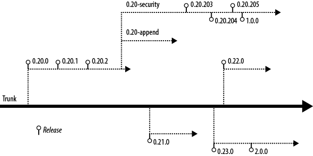
Here is a whirlwind tour of the various lines of development and their status. This information is also depicted visually in Figure 4-1.
- 0.20.0–0.20.2
The 0.20 branch of Hadoop is extremely stable and has seen quite a bit of production burn-in. This branch has been one of the longest-lived branches in Hadoop’s history since being at Apache, with the first release appearing in April 2009. CDH2 and CDH3 are both based off of this branch, albeit with many features and bug fixes from 0.21, 0.22, and 1.0 back-ported.
- 0.20-append
One of the features missing from 0.20 was support for file appends in HDFS. Apache HBase relies on the ability to sync its write ahead log, (such as force file contents to disk) which under the hood, uses the same basic functionality as file append. Append was considered a potentially destabilizing feature and many disagreed on the implementation, so it was relegated to a branch. This branch was called 0.20-append. No official release was ever made from the 0.20-append branch.
- 0.20-security
Yahoo!, one of the major contributors to Apache Hadoop, invested in adding full Kerberos support to core Hadoop. It later contributed this work back to Hadoop in the form of the 0.20-security branch, a version of Hadoop 0.20 with Kerberos authentication support. This branch would later be released as the 0.20.20X releases.
- 0.20.203–0.20.205
There was a strong desire within the community to produce an official release of Hadoop that included the 0.20-security work. The 0.20.20X releases contained not only security features from 0.20-security, but also bug fixes and improvements on the 0.20 line of development. Generally, it no longer makes sense to deploy these releases as they’re superseded by 1.0.0.
- 0.21.0
The 0.21 branch was cut from Hadoop trunk and released in August 2010. This was considered a developer preview or alpha quality release to highlight some of the features that were currently in development at the time. Despite the warning from the Hadoop developers, a small number of users deployed the 0.21 release anyway. This release does not include security, but does have append.
- 0.22.0
Hold on, because this is where the story gets weird. In December 2011, the Hadoop community released version 0.22, which was based on trunk, like 0.21 was. This release includes security, but only for HDFS. Also a bit strange, 0.22 was released after 0.23 with less functionality. This was due to when the 0.22 branch was cut from trunk.
- 0.23.0
In November 2011, version 0.23 of Hadoop was released. Also cut from trunk, 0.23 includes security, append, YARN, and HDFS federation. This release has been dubbed a developer preview or alpha-quality release. This line of development is superseded by 2.0.0.
- 1.0.0
In a continuing theme of confusion, version 1.0.0 of Hadoop was released from the 0.20.205 line of development. This means that 1.0.0 does not contain all of the features and fixes found in the 0.21, 0.22, and 0.23 releases. That said, it does include security.
- 2.0.0
In May 2012, version 2.0.0 was released from the 0.23.0 branch and like 0.23.0, is considered alpha-quality. Mainly, this is because it includes YARN and removes the traditional MRv1 jobtracker and tasktracker daemons. While YARN is API-compatible with MRv1, the underlying implementation is different enough for it to require more significant testing before being considered production-ready.
The version of Hadoop you select for deployment will ultimately be driven by the feature set you require for your applications. For many, only the releases targeted for production use are an option. This narrows the field to the 0.20, 1.0, and CDH releases almost immediately. Users who want to run HBase will also require append support.
| Feature | 0.20 | 0.21 | 0.22 | 0.23 | 1.0 | 2.0 | CDH3 | CDH4 |
|---|---|---|---|---|---|---|---|---|
| Production quality | X | X | X | X | ||||
| HDFS append | X | X | X | X | X | X | X | |
| Kerberos security | X[a] | X | X | X | X | X | X | |
| HDFS symlinks | X | X | X | X | X | |||
| YARN (MRv2) | X | X | X | |||||
| MRv1 daemons[b] | X | X | X | X | X | X | ||
| Namenode federation | X | X | X | |||||
| Namenode HA | X | X | X | |||||
[a] Support for Kerberos-enabled HDFS only. [b] All versions include support for the MRv1 APIs. | ||||||||
When planning an Hadoop cluster, picking the right hardware is critical. No one likes the idea of buying 10, 50, or 500 machines just to find out she needs more RAM or disk. Hadoop is not unlike traditional data storage or processing systems in that the proper ratio of CPU to memory to disk is heavily influenced by the workload. There are, of course, some guidelines and a reasonable base configuration, but some knowledge of the intended workload will greatly increase the likelihood of optimum utilization of the hardware.
As you probably already know, one of the major advantages of Hadoop is its ability to run on so-called commodity hardware. This isn’t just a function of cost, although that certainly plays a large role. One example of this is Hadoop’s preference for JBOD[7] and how its I/O patterns fit this model explicitly. This isn’t to say production Hadoop clusters commonly run on $1,000 machines—your expectations of what is meant by commodity may need adjustment—but rather that you won’t need to break the bank by purchasing top-end servers.
Hadoop hardware comes in two distinct classes: masters and workers. Master nodes are typically more robust to hardware failure and run critical cluster services. Loss of a master almost certainly means some kind of service disruption. On the other hand, worker nodes are expected to fail regularly. This directly impacts the type of hardware as well as the amount of money spent on these two classes of hardware. It is common that administrators, in an effort to reduce the proliferation of hardware profiles in the data center, will select a single hardware profile for all masters and a single profile for all workers. Those with deep pockets may find it even easier to purchase a single Hadoop node profile and simply ignore wasted disk on the masters, for example. There’s no single correct answer. Factors such as hardware availability, corporate standards, cost, utilization standards, and deployment profile are beyond the scope of this book. That being said, exercise good judgment and common sense and realize that strict adherence to existing standards may negate many of the benefits of Hadoop.
Note
The distinction between a node and the service assigned to said node is important. When talking about machines, there are masters and workers. These designations reflect the class of hardware. Separately, there are the five core Hadoop services: namenode, secondary namenode, datanode, jobtracker, and tasktracker, each a separate daemon. Services are run on nodes of the cluster. Worker services such as the datanode and tasktracker always run together. In smaller clusters, it sometimes makes sense to run the master services—the namenode, secondary namenode, and jobtracker—together. As the cluster grows, these services are separated and dedicated hardware for each is provisioned. When you hear “master,” the next question is always “what process?” “Slave,” or “worker,” will always mean the datanode and tasktracker pair.
For master nodes—the machines that run one or more of the namenode, jobtracker, and secondary namenode—redundancy is the name of the game. Each of these machines serves a critical function the cluster can’t live without.[8] While proponents of Hadoop beat the commodity hardware drum, this is the place where people spend more money and spring for the higher-end features. Dual power supplies, bonded network interface cards (NICs), and sometimes even RAID 10 in the case of the namenode storage device, are not uncommon to find in the wild. In general, master processes tend to be RAM-hungry but low on disk space consumption. The namenode and jobtracker are also rather adept at producing logs on an active cluster, so plenty of space should be reserved on the disk or partition on which logs will be stored.
The operating system device for master nodes should be highly available. This usually means RAID-1 (a mirrored pair of disks). Since the OS does not consume a significant amount of space, RAID-10 or RAID-5 would be overkill and lead to unusable capacity. Most of the real work is done on the data devices, while the OS device usually only has to contend with logfiles in /var/log.
Small clusters—clusters with fewer than 20 worker nodes—do not require much for master nodes in terms of hardware. A solid baseline hardware profile for a cluster of this size is a dual quad-core 2.6 Ghz CPU, 24 GB of DDR3 RAM, dual 1 Gb Ethernet NICs, a SAS drive controller, and at least two SATA II drives in a JBOD configuration in addition to the host OS device. Clusters of up to 300 nodes fall into the mid-size category and usually benefit from an additional 24 GB of RAM for a total of 48 GB. Master nodes in large clusters should have a total of 96 GB of RAM. Remember that these are baseline numbers meant to give you a place from which to start.
The namenode is absolutely critical to a Hadoop cluster and usually receives special treatment. There are three things a healthy namenode absolutely requires in order to function properly: RAM, modest but dedicated disk, and to be left alone! As we covered previously, the namenode serves all of its metadata directly from RAM. This has the obvious implication that all metadata must fit in physical memory. The exact amount of RAM required depends on how much metadata there is to maintain. Remember that the metadata contains the filename, permissions, owner and group data, list of blocks that make up each file, and current known location of each replica of each block. As you’d expect, this adds up.
There are subtleties to the namenode metadata that you might not otherwise think much about. One instance of this is that the length of filenames actually starts to matter at scale; the longer the filename, the more bytes it occupies in memory. More dubious, though, is the small files problem. Each file is made up of one or more blocks and has associated metadata. The more files the namenode needs to track, the more metadata it maintains, and the more memory it requires as a result. As a base rule of thumb, the namenode consumes roughly 1 GB for every 1 million blocks. Again, this is a guideline and can easily be invalidated by the extremes.
Namenode disk requirements are modest in terms of storage. Since all metadata must fit in memory, by definition, it can’t take roughly more than that on disk. Either way, the amount of disk this really requires is minimal—less than 1 TB.
While namenode space requirements are minimal, reliability is paramount. When provisioning, there are two options for namenode device management: use the namenode’s ability to write data to multiple JBOD devices, or write to a RAID device. No matter what, a copy of the data should always be written to an NFS (or similar) mounted volume in addition to whichever local disk configuration is selected. This NFS mount is the final hope for recovery when the local disks catch fire or when some equally unappealing, apocalyptic event occurs.[9] The storage configuration selected for production usage is usually dictated by the decision to purchase homogeneous hardware versus specially configured machines to support the master daemons. There’s no single correct answer and as mentioned earlier, what works for you depends on a great many factors.
The secondary namenode is almost always identical to the namenode. Not only does it require the same amount of RAM and disk, but when absolutely everything goes wrong, it winds up being the replacement hardware for the namenode. Future versions of Hadoop (which should be available by the time you read this) will support a highly available namenode (HA NN) which will use a pair of identical machines. When running a cluster with an HA namenode, the standby or inactive namenode instance performs the checkpoint work the secondary namenode normally does.
Similar to the namenode and secondary namenode, the jobtracker is also memory-hungry, although for a different reason. In order to provide job and task level-status, counters, and progress quickly, the jobtracker keeps metadata information about the last 100 (by default) jobs executed on the cluster in RAM. This, of course, can build up very quickly and for jobs with many tasks, can cause the jobtracker's JVM heap to balloon in size. There are parameters that allow an administrator to control what information is retained in memory and for how long, but it’s a trade-off; job details that are purged from the jobtracker’s memory no longer appear in its web UI.
Due to the way job data is retained in memory, jobtracker memory requirements can grow independent of cluster size. Small clusters that handle many jobs, or jobs with many tasks, may require more RAM than expected. Unlike the namenode, this isn’t as easy to predict because the variation in the number of tasks from job to job can be much greater than the metadata in the namenode, from file to file.
When sizing worker machines for Hadoop, there are a few points to consider. Given that each worker node in a cluster is responsible for both storage and computation, we need to ensure not only that there is enough storage capacity, but also that we have the CPU and memory to process that data. One of the core tenets of Hadoop is to enable access to all data, so it doesn’t make much sense to provision machines in such a way that prohibits processing. On the other hand, it’s important to consider the type of applications the cluster is designed to support. It’s easy to imagine use cases where the cluster’s primary function is long-term storage of extremely large datasets with infrequent processing. In these cases, an administrator may choose to deviate from the balanced CPU to memory to disk configuration to optimize for storage-dense configurations.
Starting from the desired storage or processing capacity and working backward is a technique that works well for sizing machines. Consider the case where a system ingests new data at a rate of 1 TB per day. We know Hadoop will replicate this data three times by default, which means the hardware needs to accommodate 3 TB of new data every day! Each machine also needs additional disk capacity to store temporary data during processing with MapReduce. A ballpark estimate is that 20-30% of the machine’s raw disk capacity needs to be reserved for temporary data. If we had machines with 12 × 2 TB disks, that leaves only 18 TB of space to store HDFS data, or six days' worth of data.
The same exercise can be applied to CPU and memory, although in this case, the focus is how much a machine can do in parallel rather than how much data it can store. Let’s take a hypothetical case where an hourly data processing job is responsible for processing data that has been ingested. If this job were to process 1/24th of the aforementioned 1 TB of data, each execution of the job would need to process around 42 GB of data. Commonly, data doesn’t arrive with such an even distribution throughout the day, so there must be enough capacity to be able to handle times of the day when more data is generated. This also addresses only a single job whereas production clusters generally support many concurrent jobs.
In the context of Hadoop, controlling concurrent task processing means controlling throughput with the obvious caveat of having the available processing capacity. Each worker node in the cluster executes a predetermined number of map and reduce tasks simultaneously. A cluster administrator configures the number of these slots, and Hadoop’s task scheduler—a function of the jobtracker—assigns tasks that need to execute to available slots. Each one of these slots can be thought of as a compute unit consuming some amount of CPU, memory, and disk I/O resources, depending on the task being performed. A number of cluster-wide default settings dictate how much memory, for instance, each slot is allowed to consume. Since Hadoop forks a separate JVM for each task, the overhead of the JVM itself needs to be considered as well. This means each machine must be able to tolerate the sum total resources of all slots being occupied by tasks at once.
Typically, each task needs between 2 GB and 4 GB of memory, depending on the task being performed. A machine with 48 GB of memory, some of which we need to reserve for the host OS and the Hadoop daemons themselves, will support between 10 and 20 tasks. Of course, each task needs CPU time. Now there is the question of how much CPU each task requires versus the amount of RAM it consumes. Worse, we haven’t yet considered the disk or network I/O required to execute each task. Balancing the resource consumption of tasks is one of the most difficult tasks of a cluster administrator. Later, we’ll explore the various configuration parameters available to control resource consumption between jobs and tasks.
If all of this is just too nuanced, Table 4-1 has some basic hardware configurations to start with. Note that these tend to change rapidly given the rate at which new hardware is introduced, so use your best judgment when purchasing anything.
Table 4-1. Typical worker node hardware configurations
| Midline configuration (all around, deep storage, 1 Gb Ethernet) | |
|---|---|
| CPU | 2 × 6 core 2.9 Ghz/15 MB cache |
| Memory | 64 GB DDR3-1600 ECC |
| Disk controller | SAS 6 Gb/s |
| Disks | 12 × 3 TB LFF SATA II 7200 RPM |
| Network controller | 2 × 1 Gb Ethernet |
| Notes | CPU features such as Intel’s Hyper-Threading and QPI are desirable. Allocate memory to take advantage of triple- or quad-channel memory configurations. |
| High end configuration (high memory, spindle dense, 10 Gb Ethernet) | |
|---|---|
| CPU | 2 × 6 core 2.9 Ghz/15 MB cache |
| Memory | 96 GB DDR3-1600 ECC |
| Disk controller | 2 × SAS 6 Gb/s |
| Disks | 24 × 1 TB SFF Nearline/MDL SAS 7200 RPM |
| Network controller | 1 × 10 Gb Ethernet |
| Notes | Same as the midline configuration |
Once the hardware for the worker nodes has been selected, the next obvious question is how many of those machines are required to complete a workload. The complexity of sizing a cluster comes from knowing—or more commonly, not knowing—the specifics of such a workload: its CPU, memory, storage, disk I/O, or frequency of execution requirements. Worse, it’s common to see a single cluster support many diverse types of jobs with conflicting resource requirements. Much like a traditional relational database, a cluster can be built and optimized for a specific usage pattern or a combination of diverse workloads, in which case some efficiency may be sacrificed.
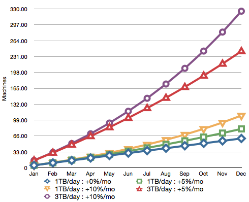
There are a few ways to decide how many machines are required for a Hadoop deployment. The first, and most common, is sizing the cluster based on the amount of storage required. Many clusters are driven by high data ingest rates; the more data coming into the system, the more machines required. It so happens that as machines are added to the cluster, we get compute resources in addition to the storage capacity. Given the earlier example of 1 TB of new data every day, a growth plan can be built that maps out how many machines are required to store the total amount of data. It usually makes sense to project growth for a few possible scenarios. For instance, Table 4-2 shows a typical plan for flat growth, 5% monthly growth, and 10% monthly growth. (See Figure 4-2.)
Table 4-2. Sample cluster growth plan based on storage
| Average daily ingest rate | 1 TB | |
| Replication factor | 3 (copies of each block) | |
| Daily raw consumption | 3 TB | Ingest × replication |
| Node raw storage | 24 TB | 12 × 2 TB SATA II HDD |
| MapReduce temp space reserve | 25% | For intermediate MapReduce data |
| Node-usable raw storage | 18 TB | Node raw storage – MapReduce reserve |
| 1 year (flat growth) | 61 nodes[a] | Ingest × replication × 365 / node raw storage |
| 1 year (5% growth per month[b]) | 81 nodes[a] | |
| 1 year (10% growth per month) | 109 nodes[a] | |
[a] Rounded to the nearest whole machine. [b] To simplify, we treat the result of the daily ingest multiplied by 365, divided by 12, as one month. Growth is compounded each month. | ||
In Table 4-2, we assume 12 × 2 TB hard drives per node, but we could have just as easily used half the number of drives per node and doubled the number of machines. This is how we can adjust the ratio of resources such as the number of CPU cores to hard drive spindles. This leads to the realization that we could purchase machines that are half as powerful and simply buy twice as many. The trade-off, though, is that doing so would require significantly more power, cooling, rack space, and network port density. For these reasons, it’s usually preferable to purchase reasonably dense machines without falling outside the normal boundaries of what is considered commodity hardware.
Projecting cluster size based on the completion time of specific jobs is less common, but still makes sense in certain circumstances. This tends to be more complicated and requires significantly more information than projections based solely on data size. Calculating the number of machines required to complete a job necessitates knowing, roughly, the amount of CPU, memory, and disk I/O used while performing a previous invocation of the same job.
There’s a clear chicken and egg problem; a job must be run with a subset of the data in order to understand how many machines are required to run the job at scale. An interesting property of MapReduce jobs is that map tasks are almost always uniform in execution. If a single map task takes one minute to execute and consumes some amount of user and system CPU time, some amount of RAM and some amount of I/O, 100 map tasks will simply take 100 times the resources. Reduce tasks, on the other hand, don’t have this property. The number of reducers is defined by the developer rather than being based on the size of the data, so it’s possible to create a situation where the job bottlenecks on the number of reducers or an uneven distribution of data between the reducers. The latter problem is referred to as reducer skew and is covered in greater detail in Chapter 9.
The large-scale data storage and processing industry moves in cycles. In the past, administrators have purchased large beefy “scale-up” machines with the goal of stuffing as much CPU, RAM, and disk into a single machine as possible. At some point, we collectively realized this was difficult and expensive. For many data center services, we moved to running “pizza boxes” and building in the notion of failure as a first-class concept. A few years later, we were confronted with another problem: many machines in the data center were drastically underutilized and the sheer number of machines was difficult to manage. This was the dawn of the great virtualization rush. Machines were consolidated onto a smaller number of beefy boxes, reducing power and improving utilization. Local disk was eschewed in favor of large storage area networks (SANs) and network attached storage (NAS) because virtual machines could now run on any physical machine in the data center. Now along comes Hadoop and everything you read says commodity, scale-out, share-nothing hardware, but what about the existing investment in blades, shared storage systems, and virtualized infrastructure?
Hadoop, generally speaking, does not benefit from virtualization. Some of the reasons concern the techniques used in modern virtualization, while others have more to do with the common practices that exist in virtualized environments. Virtualization works by running a hypervisor either in a host OS or directly on bare metal, replacing the host OS entirely. Virtual machines (VMs) can then be deployed within a hypervisor and have access to whatever hardware resources are allocated to them by the hypervisor. Historically, virtualization has hurt I/O performance-sensitive applications such as Hadoop rather significantly because guest OSes are unaware of one another as they perform I/O scheduling operations and, as a result, can cause excessive drive seek operations. Many virtualization vendors are aware of this and are working toward more intelligent hypervisors, but ultimately, it’s still slower than being directly on bare metal. For all the reasons you would not run a high-performance relational database in a VM, you should not run Hadoop in a VM.
Those new to Hadoop from the high-performance computing (HPC) space may look to use blade systems in their clusters. It is true that the density and power consumption properties of blade systems are appealing; however, the shared infrastructure between blades is generally undesirable. Blade enclosures commonly share I/O planes and network connectivity, and the blades themselves usually have little to no local storage. This is because these systems are built for compute-intensive workloads where comparatively little I/O is done. For those workloads, blade systems may be cost-effective and have a distinct advantage, but for Hadoop, they struggle to keep up.
In Worker Hardware Selection, we talked about how Hadoop prefers JBOD disk configurations. For many years—and for many systems—RAID has been dominant. There’s nothing inherently wrong with RAID; it’s fast, it’s proven, and it scales for certain types of applications. Hadoop uses disk differently. MapReduce is all about processing massive datasets, in parallel, in large sequential I/O access patterns. Imagine a machine with a single RAID-5 stripe with a stripe size of 64 KB running 10 simultaneous map tasks. Each task is going to read a 128 MB sequential block of data from disk in a series of read operations. Each read operation will be of some unknown length, dependent on the records being read and the format of the data. The problem is that even though these 10 tasks are attempting to perform sequential reads, because all I/O requests are issued to the same underlying device, the end result of interleaved reads will look like random reads, drastically reducing throughput. Contrast this with the same scenario but with 12 individual devices, each of which contains only complete 128 MB blocks. Now as I/O requests are issued by the kernel to the underlying device, it is almost certainly in the same position it was since the last read and no seek is performed. While it’s true that two map tasks could still contend for a block on a single device, the probability of that being so is significantly reduced.
Another potential pain point with RAID comes from the variation in drive rotation speed among multiple drives. Even within the same lot of drives from the same manufacturer, large variance in rotation speed can occur. In RAID, since all blocks are spread over all spindles, all operations are limited to the speed of the slowest device. In a JBOD configuration, each disk is free to spin independently and consequently, variance is less of an issue.
This brings us to shared storage systems such as SANs and NAS. Again, these systems are built with specific workloads in mind, but for Hadoop, they fall short. Keep in mind that in many ways, Hadoop was created to obviate these kinds of systems. Many of these systems put a large number of fast disks behind one or two controllers with a lot of cache. Hosts are connected to the storage system either via a SAN switch or directly, depending on the configuration. The storage system is usually drastically oversubscribed; there are many more machines connected to the disks than can possibly perform I/O at once. Even with multiple controllers and multiple HBAs per host, only a small number of machines can perform concurrent I/O. On top of the oversubscription of the controller, these systems commonly configure disks in RAID groups, which means all the problems mentioned earlier are an issue as well. This is counterintuitive in that many administrators think of SANs as being extremely fast and in many ways, scalable.
Hadoop was specifically designed to run on a large number of completely standalone commodity systems. Attempting to shoehorn it back into traditional enterprise storage and virtualization systems only results in significantly higher cost for reduced performance. Some percentage of readers will build clusters out of these components and they will work, but they will not be optimal. Exotic deployments of Hadoop usually end in exotic results, and not in a good way. You have been sufficiently warned.
While most of Hadoop is written in Java, enough native code and Linux-isms are in its surrounding infrastructure to make Linux the only production-quality option today. A significant number of production clusters run on RedHat Enterprise Linux or its freely available sister, CentOS. Ubuntu, SuSE Enterprise Linux, and Debian deployments also exist in production and work perfectly well. Your choice of operating system may be influenced by administration tools, hardware support, or commercial software support; the best choice is usually to minimize the variables and reduce risk by picking the distribution with which you’re most comfortable.
Preparing the OS for Hadoop requires a number of steps, and repeating them on a large number of machines is both time-consuming and error-prone. For this reason, it is strongly advised that a software configuration management system be used. Puppet and Chef are two open source tools that fit the bill. Extolling the virtues of these tools is beyond the scope of what can be accomplished in this section, but there’s a breadth of documentation for both to get you going. No matter what, find a configuration management suite that makes sense to you and get familiar with it. It will save you hours (or more) of tinkering and debugging down the road.
Hadoop uses a number of directories on the host filesystem. It’s important to understand what each location is for and what the growth patterns are. Some directories, for instance, are used for long-term block storage of HDFS data, and others contain temporary data while MapReduce jobs are running. Each of these directories has different security requirements as well. Later, in Chapter 5, we’ll see exactly how to configure each of these locations, but for now, it’s enough to understand that they exist.
- Hadoop home
This is the directory in which the Hadoop software is installed. Despite the name, it is commonly not installed in a user’s home directory. This directory can be made to be read only when configured correctly and usually lives in /usr/local, /opt, or /usr when Hadoop is installed via packages.
- Datanode data directories
One or more of these directories are used by the datanode to store HDFS block data. The datanode assumes that each directory provided is a separate physical device with independent spindles and round-robin blocks between disks. These directories occupy the vast majority of disk space and act as the long-term storage for data, and they are often put on the same devices as the tasktracker MapReduce local directories.
- Namenode directories
One or more of these directories are used by the namenode to store filesystem metadata. The namenode assumes that each directory provided is a separate physical device and replicates all writes to each device synchronously to ensure data availability in the event of disk failure. These directories will all require the same amount of space and generally do not use more than 100 GB. One of these directories is usually an NFS mount, so data is written off the physical machine.
- MapReduce local directories
One or more directories used by the tasktracker to store temporary data during a MapReduce job. More spindles usually means better performance as MapReduce tasks interfere with one another to a lesser degree. These directories store a moderate amount, depending on what the MapReduce job is doing, and are often put on the same devices as the datanode data directories.
- Hadoop log directory
This is a common directory used by all daemons to store log data as well as job- and task-level data. It’s normal for Hadoop to generate log data proportional to cluster usage; more MapReduce jobs means more logs.
- Hadoop pid directory
This is a directory used by all daemons to store pid files. This data is very small and doesn’t grow.
- Hadoop temp directory
Hadoop uses a temp directory for small, short-lived files it sometimes needs to create. The temp directory is most notably used on the machines from which MapReduce jobs are submitted and contains a copy of the JAR file that ultimately gets sent to the jobtracker. This is /tmp/hadoop-
<${user.name}>by default and many administrators leave it there.
Hadoop has few external software package requirements. The most critical piece of software required is the Java Development Kit (JDK). Internally, Hadoop uses many of the features introduced with Java 6, such as generics and concurrency utilities. Hadoop has surfaced bugs in every JDK on which it has been tested. To date, the Oracle (formally Sun Microsystems) HotSpot JVM is, by far, the best performing, most stable implementation available for Hadoop. That being said, the HotSpot VM has proven to be a moving target from patch to patch. Patch versions 24, 26, and 31 have been thoroughly tested and work well for production. The Hadoop community keeps a list of tested JVMs at http://wiki.apache.org/hadoop/HadoopJavaVersions where users can post their experiences with various Java VMs and versions.
All machines in the cluster should run the exact same version of Java, down to the patch level. Use of a 64-bit architecture and JDK is strongly encouraged because of the larger heap sizes required by the namenode and jobtracker. To install the JDK, follow the instructions for your OS at http://www.oracle.com/technetwork/java/javase/index-137561.html.
Note
If you choose to install Hadoop using Cloudera’s RPM packages, you will need to install Java using the Oracle RPM as well. This is because the CDH packages have a dependency on the Oracle RPM.
Beyond the JDK, there are a number of system services that will simplify the life of an administrator. This is less about Hadoop specifically and applies to general system maintenance, monitoring, and administration.
- cron
Every system needs a functioning cron daemon to drive scheduled tasks. Cleaning up temporary files, compressing old logs, and running configuration management processes are a few examples of common cluster maintenance jobs.
- ntp
The ability to correlate events on a cluster is necessary to diagnose and fix problems. One of the common gotchas is to forget to synchronize clocks between machines. Pick a node in the cluster—usually one of the master nodes—and make it a local NTP server for all other nodes. Details on configuring NTP properly are available at http://www.ntp.org/.
- ssh
Hadoop itself does not rely on SSH,[10] although it is incredibly useful for administration and debugging. Depending on the environment, developers may also have direct access to machines to view logs.
- postfix/sendmail
While nothing in Hadoop sends email, it is sometimes useful to have an MTA that supports outbound email only. This is useful for automated tasks running from cron to be able to notify administrators of exceptional circumstances. Both postfix and sendmail are fine for this purpose.
- rsync
One of the most underrated tools, rsync allows administrators to copy files efficiently locally and between hosts. If you’re not already familiar with rsync, learn it.
Let’s just get this out of the way: when it comes to host identification, discovery, and the treatment of hostnames, Hadoop is complicated and extremely picky. This topic is responsible for a fair number of cries for support on the mailing lists and almost certainly an equal amount of lost sleep on the part of many who are new to Hadoop.
But before we get into the list of things that can go wrong, let’s first talk about how Hadoop actually discovers and identifies hosts. As we discussed previously, Hadoop worker processes such as the tasktracker and datanodes heartbeat into the jobtracker and namenode (respectively) every few seconds. The first time this occurs, Hadoop learns about the worker’s existence. Part of this heartbeat includes the identity of the machine, either by hostname or by IP address. This identifier—again, either the hostname or the IP address—is how Hadoop will refer to this machine. This means that when an HDFS client, for instance, asks the namenode to open a file, the namenode will return this identifier to the client as the proper way in which to contact the worker. The exact implications of this are far-reaching; both the client and the worker now must be able to directly communicate, but the client must also be able to resolve the hostname and communicate with the worker using the identifier as it was reported to the namenode. But what name does the datanode report to the namenode? That’s the real question.
When the datanode starts up, it follows a rather convoluted process to discover the name of the machine. There are a few different configuration parameters that can affect the final decision. These parameters are covered in Chapter 5, but in its default configuration the datanode executes the following series of steps:
This seems simple enough. The only real question is what
getLocalHost() and
getCanonicalHostName() do, under the hood.
Unfortunately, this turns out to be platform-specific and sensitive to
the environment in a few ways. On Linux, with the HotSpot JVM, getLocalHost() uses
the POSIX, gethostname() which
in Linux, uses the uname() syscall. This
has absolutely no relationship to DNS or /etc/hosts, although
the name it returns is usually similar or even identical. The command
hostname, for
instance, exclusively uses gethostname() and sethostname() whereas
host and
dig use gethostbyname() and
gethostbyaddr(). The
former is how you interact with the hostname as the kernel sees it, while the
latter follows the normal Linux name resolution path.
The implementation of getLocalHost() on
Linux gets the hostname of the machine and then immediately calls
gethostbyname(). As a result, if
the hostname doesn’t resolve to an IP address, expect issues. Normally,
this isn’t a concern because there’s usually at least an entry in
/etc/hosts as a result of the
initial OS installation. Oddly enough, on Mac OS X, if the hostname doesn’t resolve, it still
returns the hostname and the IP address active on the preferred network
interface.
The second half of the equation is the implementation of
getCanonicalHostName(), which has an
interesting quirk. Hostname canonicalization is the process of finding
the complete, official, hostname according to the resolution system, in
this case, the host’s resolver library. In lay terms, this usually means
finding the fully qualified hostname. Since
getLocalHost() returns a nonqualified hostname—hadoop01 on our example
cluster—there’s some work to be done. According to the OpenJDK source
code (which may, in fact, differ from the Oracle HotSpot VM in subtle
ways), getCanonicalHostName() calls the
internal method InetAddress.getHostFromNameService(),
which gets the hostname by address via the OS resolver. What it does
next is the quirk; it gets all IP addresses for the given hostname, and
checks to make sure the original IP address appears in the list. If this
fails for any reason, including a SecurityManager
implementation that disallows resolution, the original IP address is
returned as the canonical name.
Using a simple Java[11] program, let’s examine our test cluster to see all of this in action (see Example 4-1).
Example 4-1. Java utility to display hostname information
import java.net.InetAddress;
import java.net.UnknownHostException;

public class dns {

  public static void main(String[] args) throws UnknownHostException {
    InetAddress addr = InetAddress.getLocalHost();

    System.out.println(
      String.format(
        "IP:%s hostname:%s canonicalName:%s",
        addr.getHostAddress(),       // The "default" IP address
        addr.getHostName(),          // The hostname (from gethostname())
        addr.getCanonicalHostName()  // The canonicalized hostname (from resolver)
      )
    );
  }

}
esammer@hadoop01 ~]$ hostname hadoop01 [esammer@hadoop01 ~]$ java dns IP:10.1.1.160 hostname:hadoop01 canonicalName:hadoop01.sf.cloudera.com
We can see that the hostname of the machine becomes fully qualified, as we expected. If we change the hostname of the machine to something that doesn’t resolve, things fail.
[esammer@hadoop01 ~]$ sudo hostname bananas
[sudo] password for esammer:
[esammer@hadoop01 ~]$ hostname
bananas
[esammer@hadoop01 ~]$ java dns
Exception in thread "main" java.net.UnknownHostException: bananas: bananas
        at java.net.InetAddress.getLocalHost(InetAddress.java:1354)
        at dns.main(dns.java:7)
Adding an entry to /etc/hosts
for bananas fixes the problem, but the canonical name
is the same.
[esammer@hadoop01 ~]$ cat /etc/hosts
127.0.0.1               localhost.localdomain localhost

10.1.1.160 hadoop01.sf.cloudera.com hadoop01 bananas
10.1.1.161 hadoop02.sf.cloudera.com hadoop02
# Other hosts...
[esammer@hadoop01 ~]$ java dns
IP:10.1.1.160 hostname:bananas canonicalName:hadoop01.sf.cloudera.com
Moving bananas to the “canonical name” position
in the hosts file changes the result.[12]
[esammer@hadoop01 ~]$ java dns
IP:10.1.1.160 hostname:bananas canonicalName:bananas
[esammer@hadoop01 ~]$ cat /etc/hosts
127.0.0.1               localhost.localdomain localhost

10.1.1.160 bananas hadoop01.sf.cloudera.com hadoop01
10.1.1.161 hadoop02.sf.cloudera.com hadoop02
# Other hosts...
This is all well and good, but what could really go wrong? After all, hostnames are just hostnames. Unfortunately, it’s not that simple. There are a few pathological cases where seemingly benign (and worse, common) configuration leads to very unexpected results.
One of the most common issues is that the machine believes its name to be 127.0.01. Worse, some versions of CentOS and RHEL configure things this way by default! This is extremely dangerous because datanodes communicate to the namenode that they’re alive and well, but they report their IP address to be 127.0.0.1 or localhost, which, in turn, is given to clients attempting to read or write data to the cluster. The clients are told to write to the datanode at 127.0.0.1—in other words, themselves—and they constantly fail. This goes down as one of the worst configuration mistakes that can occur because neither traditional monitoring tools nor the untrained administrator will notice this until it’s far too late. Even then, it still may not be clear why the machine reports itself this way.
[esammer@hadoop01 ~]$ cat /etc/hosts
127.0.0.1               localhost.localdomain localhost bananas

10.1.1.160 hadoop01.sf.cloudera.com hadoop01
10.1.1.161 hadoop02.sf.cloudera.com hadoop02
# Other hosts...
[esammer@hadoop01 ~]$ java dns
IP:127.0.0.1 hostname:bananas canonicalName:localhost.localdomain
Hadoop is, in many ways, an arbitrary code execution engine. Users submit code in the form of MapReduce jobs to the cluster, which is instantiated and executed on worker nodes within the cluster. To mitigate obvious attack vectors and protect potentially sensitive data, it’s advisable to run HDFS daemons as one user and MapReduce daemons as another. MapReduce jobs, in turn, execute either as the same user as the tasktracker daemon or as the user that submitted the job (see Table 4-3). The latter option is only available when a cluster is operating in so-called secure mode.
Historically, it was common to run all daemons as a single user,
usually named hadoop.
This was prior to support for secure operation being a first class
deployment mode and suffered from potential data exposure issues. For
example, if a MapReduce task is running as user hadoop, that process can simply open
raw blocks on the worker’s Linux filesystem, bypassing all application-level
authorization checks. By running child tasks as user mapred the standard filesystem access
controls can be used to restrict direct access to datanode block data.
For more information about user identity, authentication, and
authorization in MapReduce see Chapter 6.
By default, the CDH Hadoop RPM and Deb packages will create these users if they don’t already exist, and the init scripts will start the daemons as the correct users. Users of Apache Hadoop can write similar scripts or use an external system to ensure daemons are started as the correct users.
Each Hadoop daemon consumes various system resources, as you can guess. Linux supports, via Pluggable Authentication Modules (PAM) system, the ability to control resources such as file descriptors and virtual memory at the user level. These resource limits are defined in /etc/security/limits.conf or as fragment files in the /etc/security/limits.d directory, and affect all new logins. The format of the file isn’t hard to understand, as shown in Example 4-2.
Example 4-2. Sample limits.conf for Hadoop
# Allow users hdfs, mapred, and hbase to open 32k files. The
# type '-' means both soft and hard limits.
#
# See 'man 5 limits.conf' for details.

# user type   resource  value

hdfs   -      nofile    32768
mapred -      nofile    32768
hbase  -      nofile    32768
Each daemon uses different reserved areas of the local filesystem to store various types of data, as shown in Table 4-4. Chapter 5 covers how to define the directories used by each daemon.
Table 4-4. Hadoop directories and permissions
| Daemon | Sample path(s) | Configuration parameter | Owner:Group | Permissions |
|---|---|---|---|---|
| Namenode | /data/1/dfs/nn,/data/2/dfs/nn,/data/3/dfs/nn | dfs.name.dir | hdfs:hadoop | 0700 |
| Secondary namenode | /data/1/dfs/snn | fs.checkpoint.dir | hdfs:hadoop | 0700 |
| Datanode | /data/1/dfs/dn,/data/2/dfs/dn,/data/3/dfs/dn,/data/4/dfs/dn | dfs.datanode.dir | hdfs:hadoop | 0700 |
| Tasktracker | /data/1/mapred/local,/data/2/mapred/local,/data/3/mapred/local,/data/4/mapred/local | mapred.local.dir | mapred:hadoop | 0770 |
| Jobtracker | /data/1/mapred/local | mapred.local.dir | mapred:hadoop | 0700 |
| All | /var/log/hadoop | $HADOOP_LOG_DIR | root:hadoop | 0775
[a] |
/tmp/hadoop-user.name | hadoop.tmp.dir | root:root | 1777 | |
[a] Optionally | ||||
These directories should be created with the proper permissions prior to deploying Hadoop. Users of Puppet or Chef usually create a Hadoop manifest or recipe, respectively, that ensures proper directory creation during host provisioning. Note that incorrect permissions or ownership of directories can result in daemons that don’t start, ignored devices, or accidental exposure of sensitive data. When operating in secure mode, some of the daemons validate permissions on critical directories and will refuse to start if the environment is incorrectly configured.
There are a few kernel parameters that are of special interest when deploying Hadoop. Since production Hadoop clusters always have dedicated hardware, it makes sense to tune the OS based on what we know about how Hadoop works. Kernel parameters should be configured in /etc/sysctl.conf so that settings survive reboots.
The kernel parameter vm.swappiness controls the kernel’s
tendency to swap application data from memory to disk, in contrast to
discarding filesystem cache. The valid range for vm.swappiness is 0 to 100 where higher
values indicate that the kernel should be more aggressive in swapping
application data to disk, and lower values defer this behavior, instead
forcing filesystem buffers to be discarded. Swapping Hadoop daemon data
to disk can cause operations to timeout and potentially fail if the disk is performing
other I/O operations. This is especially dangerous for HBase as Region
Servers must maintain communication with ZooKeeper lest they be marked
as failed. To avoid this, vm.swappiness should be set to 0 (zero)
to instruct the kernel to never swap application data, if there is an
option. Most Linux distributions ship with vm.swappiness set to 60 or even as high
as 80.
Processes commonly allocate memory by calling the
function malloc().
The kernel decides if enough RAM is available and either grants or
denies the allocation request. Linux (and a few other Unix variants)
support the ability to overcommit memory; that is, to permit more memory
to be allocated than is available in physical RAM plus swap. This is
scary, but sometimes it is necessary since applications commonly
allocate memory for “worst case” scenarios but never use it.
There are three possible settings for vm.overcommit_memory.
- 0 (zero)
Check if enough memory is available and, if so, allow the allocation. If there isn’t enough memory, deny the request and return an error to the application.
- 1 (one)
Permit memory allocation in excess of physical RAM plus swap, as defined by
vm.overcommit_ratio. Thevm.overcommit_ratioparameter is a percentage added to the amount of RAM when deciding how much the kernel can overcommit. For instance, avm.overcommit_ratioof 50 and 1 GB of RAM would mean the kernel would permit up to 1.5 GB, plus swap, of memory to be allocated before a request failed.- 2 (two)
The kernel’s equivalent of “all bets are off,” a setting of 2 tells the kernel to always return success to an application’s request for memory. This is absolutely as weird and scary as it sounds.
When a process forks, or calls the fork() function, its entire page table is
cloned. In other words, the child process has a complete copy of the
parent’s memory space, which requires, as you’d expect, twice the amount
of RAM. If that child’s intention is to immediately call exec() (which replaces one process with
another) the act of cloning the parent’s memory is a waste of time.
Because this pattern is so common, the vfork() function was
created, which unlike fork(), does
not clone the parent memory, instead blocking it until the child either
calls exec() or exits. The problem
is that the HotSpot JVM developers implemented Java’s fork operation
using fork() rather than vfork().
So why does this matter to Hadoop? Hadoop Streaming—a library that allows MapReduce jobs to
be written in any language that can read from standard in and write to
standard out—works by forking the user’s code as a child process and
piping data through it. This means that not only do we need to account
for the memory the Java child task uses, but also that when it forks,
for a moment in time before it execs, it uses twice the amount of memory
we’d expect it to. For this reason, it is sometimes necessary to set
vm.overcommit_memory to
the value 1 (one) and adjust vm.overcommit_ratio accordingly.
Disk configuration and performance is extremely important to Hadoop. Since many kinds of MapReduce jobs are I/O-bound, an underperforming or poorly configured disk can drastically reduce overall job performance. Datanodes store block data on top of a traditional filesystem rather than on raw devices. This means all of the attributes of the filesystem affect HDFS and MapReduce, for better or worse.
Today Hadoop primarily runs on Linux: as a result we’ll focus on common Linux filesystems. To be sure, Hadoop can run on more exotic filesystems such as those from commercial vendors, but this usually isn’t cost-effective. Remember that Hadoop is designed to be not only low-cost, but also modest in its requirements on the hosts on which it runs. By far, the most common filesystems used in production clusters are ext3, ext4, and xfs.
As an aside, the Linux Logical Volume Manager (LVM) should never be used for Hadoop data disks. Unfortunately, this is the default for CentOS and RHEL when using automatic disk allocation during installation. There is obviously a performance hit when going through an additional layer such as LVM between the filesystem and the device, but worse is the fact that LVM allows one to concatenate devices into larger devices. If you’re not careful during installation, you may find that all of your data disks have been combined into a single large device without any protection against loss of a single disk. The dead giveaway that you’ve been bitten by this unfortunate configuration mishap is that your device name shows up as /dev/vg* or something other than /dev/sd*.
Warning
The commands given here will format disks. Formatting a disk is a destructive operation and will destroy any existing data on the disk. Do not format a disk that contains data you need!
The third extended filesystem, or ext3, is an enhanced version of ext2. The most notable feature of ext3 is support for journaling, which records changes in a journal or log prior to modifying the actual data structures that make up the filesystem. Ext3 has been included in Linux since kernel version 2.4.15 and has significant production burn-in. It supports files up to 2 TB and a max filesystem size of 16 TB when configured with a 4 KB block size. Note that the maximum filesystem size is less of a concern with Hadoop because data is written across many machines and many disks in the cluster. Multiple journal levels are supported, although ordered mode, where the journal records metadata changes only, is the most common. If you’re not sure what filesystem to use, or you’re extremely risk-averse, ext3 is for you.
When formatting devices for ext3, the following options are worth specifying:
mkfs -t ext3 -j -m 1 -O sparse_super,dir_index /dev/sdXNThe option -t
ext3 simply tells mkfs to
create an ext3 filesystem while -j enables the journal. The
-m1 option is a
hidden gem and sets the percentage of reserved blocks for the
superuser to 1% rather than 5%. Since no root processes should be
touching data disks, this leaves us with an extra 4% of usable disk
space. With 2 TB disks, that’s up to 82 GB! Additional options to the
filesystem are specified by the -O option. Admittedly, the two
options shown—sparse_super, which creates fewer
super-block backups, and dir_index, which uses b-tree
indexes for directory trees for faster lookup of files in large
directories—are almost certainly the defaults on your Linux distro of
choice. Of course, /dev/sd specifies the
device to format, where XNXN
Ext4 is the successor to ext3; it was released as of Linux 2.6.28 and contains some desirable improvements. Specifically, ext4 is extent-based, which improves sequential performance by storing contiguous blocks together in a larger unit of storage. This is especially interesting for Hadoop, which is primarily interested in reading and writing data in larger blocks. Another feature of ext4 is journal checksum calculation; a feature that improves data recoverability in the case of failure during a write. Newer Linux distributions such as RedHat Enterprise Linux 6 (RHEL6) will use ext4 as the default filesystem unless configured otherwise.
All of this sounds great, but ext4 has a major drawback: burn-in
time. Only now is ext4 starting to see significant deployment in
production systems. This can be disconcerting to those that are
risk-averse. The following format command is similar to that of ext3,
except we add the extent argument to the
-O option to enable the use of extent-based
allocation:
mkfs -t ext4 -m 1 -O dir_index,extent,sparse_super /dev/sdXNXFS, a filesystem created by SGI, has a number of unique features. Like ext3 and ext4, it’s a journaling filesystem, but the way data is organized on disk is very different. Similar to ext4, allocation is extent-based, but its extents are within allocation groups, each of which is responsible for maintaining its own inode table and space. This model allows concurrent operations in a way that ext3 and 4 cannot, because multiple processes can modify data in each allocation group without conflict. Its support for high concurrency makes xfs very appealing for systems such as relational databases that perform many parallel, but short-lived, operations.
mkfs -t xfs /dev/sdXNThere are no critical options to creating xfs filesystems for Hadoop.
After filesystems have been formatted, the next step is to add an entry for each newly formatted filesystem to the system's /etc/fstab file, as shown in Example 4-3. The reason this somewhat mundane task is called out is because there’s an important optimization to be had: disabling file access time. Most filesystems support the notion of keeping track of the access time of both files and directories. For desktops, this is a useful feature; it’s easy to figure out what files you’ve most recently viewed as well as modified. This feature isn’t particularly useful in the context of Hadoop. Users of HDFS are, in many cases, unaware of the block boundaries of files, so the fact that block two of file foo was accessed last week is of little value. The real problem with maintaining access time (or atime as it’s commonly called) is that every time a file is read, the metadata needs to be updated. That is, for each read, there’s also a mandatory write. This is relatively expensive at scale and can negatively impact the overall performance of Hadoop, or any other system, really. When mounting data partitions, it’s best to disable both file atime and directory atime.
Example 4-3. Sample /etc/fstab file
LABEL=/         /          ext3    noatime,nodiratime        1 1
LABEL=/data/1   /data/1    ext3    noatime,nodiratime        1 2
LABEL=/data/2   /data/2    ext3    noatime,nodiratime        1 2
LABEL=/data/3   /data/3    ext3    noatime,nodiratime        1 2
LABEL=/data/4   /data/4    ext3    noatime,nodiratime        1 2
tmpfs           /dev/shm   tmpfs   defaults        0 0
devpts          /dev/pts   devpts  gid=5,mode=620  0 0
sysfs           /sys       sysfs   defaults        0 0
proc            /proc      proc    defaults        0 0
LABEL=SWAP-sda2 swap       swap    defaults        0 0
Network design and architecture is a complex, nuanced topic on which many books have been written. This is absolutely not meant to be a substitute for a complete understanding of such a deep subject. Instead, the goal is to highlight what elements of network design are crucial from the perspective of Hadoop deployment and performance.
The following sections assume you’re already familiar with basic networking concepts such as the OSI model, Ethernet standards such as 1- (1GbE) and 10-gigabit (10GbE), and the associated media types. Cursory knowledge of advanced topics such as routing theory and at least one protocol such as IS-IS, OSPF, or BGP is helpful in getting the most out of Spine fabric. In the interest of simplicity, we don’t cover bonded hosts or switch redundancy where it’s obviously desirable. This isn’t because it’s not important, but because how you accomplish that tends to get into switch-specific features and vendor-supported options.
Hadoop was developed to exist and thrive in real-world network topologies. It doesn’t require any specialized hardware, nor does it employ exotic network protocols. It will run equally well in both flat Layer 2 networks or routed Layer 3 environments. While it does attempt to minimize the movement of data around the network when running MapReduce jobs, there are times when both HDFS and MapReduce generate considerable traffic. Rack topology information is used to make reasonable decisions about data block placement and to assist in task scheduling, but it helps to understand the traffic profiles exhibited by the software when planning your cluster network.
In Chapter 2, we covered the nuts and bolts of how HDFS works and why. Taking a step back and looking at the system from the perspective of the network, there are three primary forms of traffic: cluster housekeeping traffic such as datanode block reports and heartbeats to the namenode, client metadata operations with the namenode, and block data transfer. Basic heartbeats and administrative commands are infrequent and only transfer small amounts of data in remote procedure calls. Only in extremely large cluster deployments—on the order of thousands of machines—does this traffic even become noticeable.
Most administrators will instead focus on dealing with the rate of data being read from, or written to, HDFS by client applications. Remember, when clients that execute on a datanode where the block data is stored perform read operations, the data is read from the local device, and when writing data, they write the first replica to the local device. This reduces a significant amount of network data transfer. Clients that do not run on a datanode or that read more than a single block of data will cause data to be transferred across the network. Of course, with a traditional NAS device, for instance, all data moves across the network, so anything HDFS can do to mitigate this is already an improvement, but it’s nothing to scoff at. In fact, writing data from a noncollocated client causes the data to be passed over the network three times, two of which pass over the core switch in a traditional tree network topology. This replication traffic moves in an East/West pattern rather than the more common client/server-oriented North/South. Significant East/West traffic is one of the ways Hadoop is different from many other traditional systems.
Beyond normal client interaction with HDFS, failures can also generate quite a bit of traffic. Much simpler to visualize, consider what happens when a datanode that contains 24 TB of block data fails. The resultant replication traffic matches the amount of data contained on the datanode when it failed.
It’s no surprise that the MapReduce cluster membership and heartbeat infrastructure matches that of HDFS. Tasktrackers regularly heartbeat small bits of information to the jobtracker to indicate they’re alive. Again, this isn’t a source of pain for most administrators, save for the extreme scale cases. Client applications also do not communicate directly with tasktrackers, instead performing most operations against the jobtracker and HDFS. During job submission, the jobtracker communicates with the namenode, but also in the form of small RPC requests. The true bear of MapReduce is the tasktracker traffic during the shuffle phase of a MapReduce job.
As map tasks begin to complete and reducers are started, each reducer must fetch the map output data for its partition from each tasktracker. Performed by HTTP, this results in a full mesh of communication; each reducer (usually) must copy some amount of data from every other tasktracker in the cluster. Additionally, each reducer is permitted a certain number of concurrent fetches. This shuffle phase accounts for a rather significant amount of East/West traffic within the cluster, although it varies in size from job to job. A data processing job, for example, that transforms every record in a dataset will typically transform records in map tasks in parallel. The result of this tends to be a different record of roughly equal size that must be shuffled, passed through the reduce phase, and written back out to HDFS in its new form. A job that transforms an input dataset of 1 million 100 KB records (roughly 95 GB) to a dataset of one million 82 KB records (around 78 GB) will shuffle at least 78 GB over the network for that job alone, not to mention the output from the reduce phase that will be replicated when written to HDFS.
Remember that active clusters run many jobs at once and typically must continue to take in new data being written to HDFS by ingestion infrastructure. In case it’s not clear, that’s a lot of data.
Frequently, when discussing Hadoop networking, users will ask if they should deploy 1 Gb or 10 Gb network infrastructure. Hadoop does not require one or the other; however, it can benefit from the additional bandwidth and lower latency of 10 Gb connectivity. So the question really becomes one of whether the benefits outweigh the cost. It’s hard to truly evaluate cost without additional context. Vendor selection, network size, media, and phase of the moon all seem to be part of the pricing equation. You have to consider the cost differential of the switches, the host adapters (as 10 GbE LAN on motherboard is still not yet pervasive), optics, and even cabling, to decide if 10 Gb networking is feasible. On the other hand, plenty of organizations have simply made the jump and declared that all new infrastructure must be 10 Gb, which is also fine. Estimates, at the time of publication, are that a typical 10 Gb top of rack switch is roughly three times more expensive than its 1 Gb counterpart, port for port.
Those that primarily run ETL-style or other high input to output data ratio MapReduce jobs may prefer the additional bandwidth of a 10 Gb network. Analytic MapReduce jobs—those that primarily count or aggregate numbers—perform far less network data transfer during the shuffle phase, and may not benefit at all from such an investment. For space- or power-constrained environments, some choose to purchase slightly beefier hosts with more storage that, in turn, require greater network bandwidth in order to take full advantage of the hardware. The latency advantages of 10 Gb may also benefit those that wish to run HBase to serve low-latency, interactive applications. Finally, if you find yourself considering bonding more than two 1 Gb interfaces, you should almost certainly look to 10 Gb as, at that point, the port-for-port cost starts to become equivalent.
It’s impossible to fully describe all possible network topologies here. Instead, we focus on two: a common tree, and a spine/leaf fabric that is gaining popularity for applications with strong East/West traffic patterns.
By far, the N-tiered tree network (see Figure 4-3) is the predominant architecture deployed in data centers today. A tree may have multiple tiers, each of which brings together (or aggregates) the branches of another tier. Hosts are connected to leaf or access switches in a tree, which are then connected via one or more uplinks to the next tier. The number of tiers required to build a network depends on the total number of hosts that need to be supported. Using a switch with 48 1GbE and four 10GbE port switches as an access switch, and a 48-port 10GbE switch as a distribution switch, it’s possible to support up to 576 hosts (because each access switch uses 4-ports of the 48-port distribution switch).
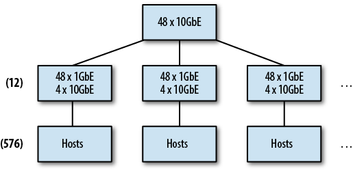
Notice that the sum of the four 10GbE uplinks from each distribution switch can’t actually support the full bandwidth of the 48 1GbE ports. This is referred to as oversubscription of the bandwidth. In simpler terms, it’s not possible for all 48 hosts to communicate at the full, advertised rate of the port to which they are connected. Oversubscription is commonly expressed as a ratio of the amount of desired bandwidth required versus bandwidth available. In our example, the 48 1GbE ports can theoretically carry 48 Gb of traffic, but the four 10GbE ports only support 40 Gb. Dividing the desired bandwidth (48) by the available bandwidth (40) yields an oversubscription ratio of 1.2:1. It’s very common for some amount of oversubscription to occur at the uplink of one tier to the next in a tree. This is one of the primary reasons why Hadoop tries to keep network activity confined to a single rack, or switch, really.
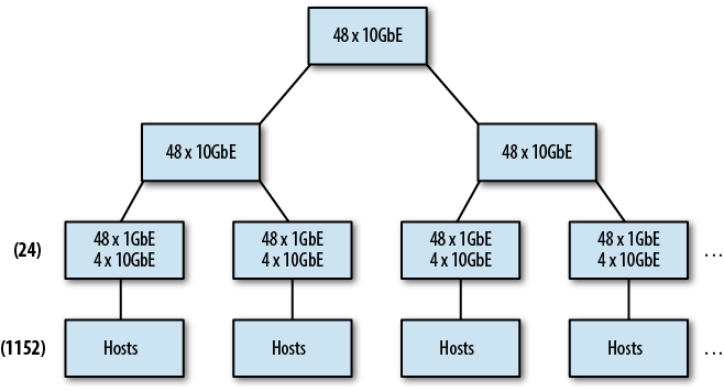
What happens, though, when we run out of ports at the distribution switch? At some point, it becomes either cost-prohibitive or simply impossible to buy switches with more ports. In a tree, the answer is to add another tier of aggregation. The problem with this is that each time you add a tier, you increase the number of switches between some nodes and others. Worse, the amount of oversubscription is compounded with each tier in the tree. Consider what happens if we extend our tree network from earlier beyond 576 hosts. To increase our port density any further we must create a third tier (see Figure 4-4). The problem now becomes the oversubscription between tiers two and three. With 576 Gb of traffic at each tier two switch, we won’t be able to maintain the 1.2:1 oversubscription rate; that would require roughly 48 10GbE or 12 40GbE uplink ports per distribution switch. With each tier that is added, oversubscription worsens, and creates wildly different bandwidth availability between branches of the tree. As we’ve seen, Hadoop does its best to reduce interswitch communication during some operations, but others cannot be avoided, leading to frequent, and sometimes severe, contention at these oversubscribed choke points in the network. Ultimately, most network administrators come to the conclusion that a modular chassis switch that supports high port density is the answer to this problem. Beefy modular switches such as the Cisco Nexus 7000 series are not unusual to find in large tree networks supporting Hadoop clusters, but they can be expensive and can simply push the problem out until you run out of ports again. For large clusters, this is not always sufficient.
If we look instead at the North/South traffic support, a tree makes a lot of sense. Traffic enters via the root of the tree and is, by definition, limited to the capacity of the root itself. This traffic never traverses more than one branch and is far simpler to handle as a result.
It’s worth noting that cluster data ingress and egress should be nearest to the root of a tree network. This prevents branch monopolization and unbalanced traffic patterns that negatively impact some portions of the network and not others. Placing the border of the cluster at the cluster’s core switch makes this traffic equidistant to all nodes in the tree and amortizes the bandwidth cost over all branches equally.
A tree network works for small and midsize networks that fit within two tiers with minimal oversubscription. Typical access switches for a 1GbE network tend to be 48 ports with four 10GbE uplinks to a distribution layer. The distribution switch size depends on how many nodes need to be supported, but 48-port 10GbE switches are common. If you are tacking Hadoop onto an existing tree, bring the cluster’s distribution layer in nearest to that of ETL, process orchestration, database, or other systems with which you plan to exchange data. Do not, under any circumstances, place low-latency services on the cluster distribution switch. Hadoop tends to monopolize shared resources such as buffers, and can (and will) create problems for other hosts.
Over the past few years, general purpose virtualized infrastructure and large-scale data processing clusters have grown in popularity. These types of systems have very different traffic patterns from traditional systems in that they both require significantly greater East/West bandwidth. We’ve already discussed Hadoop’s traffic patterns, but in many ways it’s similar to that of a virtualized environment. In a true virtualized environment, applications relinquish explicit control over physical placement in exchange for flexibility and dynamism. Implicitly, this means that two applications that may need high-bandwidth communication with each other could be placed on arbitrary hosts, and by extension, switches, in the network. While it’s true that some virtualization systems support the notion of locality groups that attempt to place related virtual machines “near” one another, it’s usually not guaranteed, nor is it possible to ensure you’re not placed next to another high-traffic application. A new type of network design is required to support this new breed of systems.
Enter the scale-out spine fabric, seen in Figure 4-5. As its name implies, a fabric looks more like a tightly weaved mesh with as close to equal distance between any two hosts as possible. Hosts are connected to leaf switches, just as in the tree topology; however, each leaf has one or more uplinks to every switch in the second tier, called the spine. A routing protocol such as IS-IS, OSPF, or EIGRP is run with equal cost multipath (ECMP) routes so that traffic has multiple path options and takes the shortest path between two hosts. If each leaf has an uplink to each spine switch, every host (that isn’t on the same leaf) is always exactly three hops away. This equidistant, uniform bandwidth configuration is perfect for applications with strong East/West traffic patterns. Using the same example as earlier, converting our two distribution switches to a spine, it’s possible to support 24-leaf switches or 1,152 hosts at the same 1.2:1 oversubscription rate.
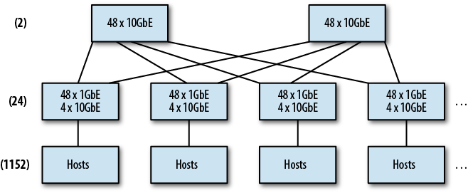
In a fabric, it’s not uncommon to use more and more ports on each leaf to support a wider spine for greater port density. To give you an idea of how this scales, four 48-port 10GbE spine switches will support forty-eight 48-port 1GbE leaf switches at the same 1.2:1 oversubscription rate for a total of 2,304 1GbE ports, as shown in Figure 4-6. That’s not a typo. Each leaf switch has one uplink to each of the four spine switches with 48 1GbE ports for host connectivity. It’s safe to reduce the number of uplinks from leaf to spine because ECMP routing says we can simply take a different path to the same place; the bandwidth isn’t gone, just spread out. Scaling out further is possible by increasing the number of spine switches and uplinks per leaf. For leaf switches with only four 10GbE ports things get a little complicated, but it’s possible to buy switches with two 40GbE QSFP+ ports to overcome this. Using a breakout cable, it’s possible to use each 40GbE QSFP+ port as four 10GbE ports for up to eight uplinks. Beyond eight spine switches (which, by the way, is 96 leaf switches or 4,608 1GbE ports), it’s usually necessary to go to 10GbE leaf switches to support additional uplinks. We then start taking away ports for hosts on each leaf and using them for uplinks, but it still allows larger and larger networks. Some Hadoop community members have written, at length, about the port density, bandwidth, cost, and power concerns when building large-scale fabrics; Brad Hedlund has an amazing blog where he regularly talks about building large-scale networks for Hadoop and OpenStack deployments.
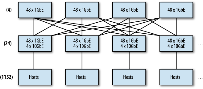
Cluster access in a spine fabric can be placed on a dedicated leaf. Since all leaves have equidistant access to all others via the spine, bandwidth is not sacrificed. Also noteworthy is that the spine fabric implicitly supports redundancy because of the use of ECMP routing. It’s possible to lose up N – 1 spine switches where N is the number of uplinks per leaf, although bandwidth is obviously reduced with each loss as well.
[7] Just a bunch of disks; a disk configuration where individual disks are accessed directly by the operating system without the need for RAID.
[8] ...or at least not for long.
[9] Almost certainly, and without fail, a human will be the demise of your namenode should you not heed the warning to leave it alone.
[10] Some of the supporting shell scripts do use ssh to start and stop services on the cluster.
[11] This code can be compiled and run using javac dns.java followed by
java
          dns
.
[12] See man 5 hosts for details on the difference between fields two and three in the hosts file.
Get Hadoop Operations now with the O’Reilly learning platform.
O’Reilly members experience books, live events, courses curated by job role, and more from O’Reilly and nearly 200 top publishers.

