High Performance Python, 2nd Edition

Chapter 1. Understanding Performant Python

Questions You’ll Be Able to Answer After This Chapter

• What are the elements of a computer’s architecture?

• What are some common alternate computer architectures?

• How does Python abstract the underlying computer architecture?

• What are some of the hurdles to making performant Python code?

• What strategies can help you become a highly performant programmer?

Programming computers can be thought of as moving bits of data and transforming them in special ways to achieve a particular result. However, these actions have a time cost. Consequently, high performance programming can be thought of as the act of minimizing these operations either by reducing the overhead (i.e., writing more efficient code) or by changing the way that we do these operations to make each one more meaningful (i.e., finding a more suitable algorithm).

Let’s focus on reducing the overhead in code in order to gain more insight into the actual hardware on which we are moving these bits. This may seem like a futile exercise, since Python works quite hard to abstract away direct interactions with the hardware. However, by understanding both the best way that bits can be moved in the real hardware and the ways that Python’s abstractions force your bits to move, you can make progress toward writing high performance programs in Python.

The Fundamental Computer System

The underlying components that make up a computer can be simplified into three basic parts: the computing units, the memory units, and the connections between them. In addition, each of these units has different properties that we can use to understand them. The computational unit has the property of how many computations it can do per second, the memory unit has the properties of how much data it can hold and how fast we can read from and write to it, and finally, the connections have the property of how fast they can move data from one place to another.

Using these building blocks, we can talk about a standard workstation at multiple levels of sophistication. For example, the standard workstation can be thought of as having a central processing unit (CPU) as the computational unit, connected to both the random access memory (RAM) and the hard drive as two separate memory units (each having different capacities and read/write speeds), and finally a bus that provides the connections between all of these parts. However, we can also go into more detail and see that the CPU itself has several memory units in it: the L1, L2, and sometimes even the L3 and L4 cache, which have small capacities but very fast speeds (from several kilobytes to a dozen megabytes). Furthermore, new computer architectures generally come with new configurations (for example, Intel’s SkyLake CPUs replaced the frontside bus with the Intel Ultra Path Interconnect and restructured many connections). Finally, in both of these approximations of a workstation we have neglected the network connection, which is effectively a very slow connection to potentially many other computing and memory units!

To help untangle these various intricacies, let’s go over a brief description of these fundamental blocks.

Computing Units

The computing unit of a computer is the centerpiece of its usefulness—it provides the ability to transform any bits it receives into other bits or to change the state of the current process. CPUs are the most commonly used computing unit; however, graphics processing units (GPUs) are gaining popularity as auxiliary computing units. They were originally used to speed up computer graphics but are becoming more applicable for numerical applications and are useful thanks to their intrinsically parallel nature, which allows many calculations to happen simultaneously. Regardless of its type, a computing unit takes in a series of bits (for example, bits representing numbers) and outputs another set of bits (for example, bits representing the sum of those numbers). In addition to the basic arithmetic operations on integers and real numbers and bitwise operations on binary numbers, some computing units also provide very specialized operations, such as the “fused multiply add” operation, which takes in three numbers, A, B, and C, and returns the value A * B + C.

The main properties of interest in a computing unit are the number of operations it can do in one cycle and the number of cycles it can do in one second. The first value is measured by its instructions per cycle (IPC),¹ while the latter value is measured by its clock speed. These two measures are always competing with each other when new computing units are being made. For example, the Intel Core series has a very high IPC but a lower clock speed, while the Pentium 4 chip has the reverse. GPUs, on the other hand, have a very high IPC and clock speed, but they suffer from other problems like the slow communications that we discuss in “Communications Layers”.

Furthermore, although increasing clock speed almost immediately speeds up all programs running on that computational unit (because they are able to do more calculations per second), having a higher IPC can also drastically affect computing by changing the level of vectorization that is possible. Vectorization occurs when a CPU is provided with multiple pieces of data at a time and is able to operate on all of them at once. This sort of CPU instruction is known as single instruction, multiple data (SIMD).

In general, computing units have advanced quite slowly over the past decade (see Figure 1-1). Clock speeds and IPC have both been stagnant because of the physical limitations of making transistors smaller and smaller. As a result, chip manufacturers have been relying on other methods to gain more speed, including simultaneous multithreading (where multiple threads can run at once), more clever out-of-order execution, and multicore architectures.

Hyperthreading presents a virtual second CPU to the host operating system (OS), and clever hardware logic tries to interleave two threads of instructions into the execution units on a single CPU. When successful, gains of up to 30% over a single thread can be achieved. Typically, this works well when the units of work across both threads use different types of execution units—for example, one performs floating-point operations and the other performs integer operations.

Out-of-order execution enables a compiler to spot that some parts of a linear program sequence do not depend on the results of a previous piece of work, and therefore that both pieces of work could occur in any order or at the same time. As long as sequential results are presented at the right time, the program continues to execute correctly, even though pieces of work are computed out of their programmed order. This enables some instructions to execute when others might be blocked (e.g., waiting for a memory access), allowing greater overall utilization of the available resources.

Finally, and most important for the higher-level programmer, there is the prevalence of multicore architectures. These architectures include multiple CPUs within the same unit, which increases the total capability without running into barriers to making each individual unit faster. This is why it is currently hard to find any machine with fewer than two cores—in this case, the computer has two physical computing units that are connected to each other. While this increases the total number of operations that can be done per second, it can make writing code more difficult!

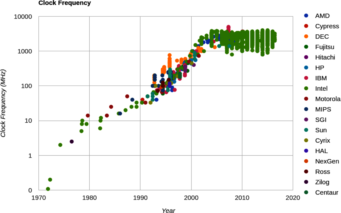
Figure 1-1. Clock speed of CPUs over time (from CPU DB)

Simply adding more cores to a CPU does not always speed up a program’s execution time. This is because of something known as Amdahl’s law. Simply stated, Amdahl’s law is this: if a program designed to run on multiple cores has some subroutines that must run on one core, this will be the limitation for the maximum speedup that can be achieved by allocating more cores.

For example, if we had a survey we wanted one hundred people to fill out, and that survey took 1 minute to complete, we could complete this task in 100 minutes if we had one person asking the questions (i.e., this person goes to participant 1, asks the questions, waits for the responses, and then moves to participant 2). This method of having one person asking the questions and waiting for responses is similar to a serial process. In serial processes, we have operations being satisfied one at a time, each one waiting for the previous operation to complete.

However, we could perform the survey in parallel if we had two people asking the questions, which would let us finish the process in only 50 minutes. This can be done because each individual person asking the questions does not need to know anything about the other person asking questions. As a result, the task can easily be split up without having any dependency between the question askers.

Adding more people asking the questions will give us more speedups, until we have one hundred people asking questions. At this point, the process would take 1 minute and would be limited simply by the time it takes a participant to answer questions. Adding more people asking questions will not result in any further speedups, because these extra people will have no tasks to perform—all the participants are already being asked questions! At this point, the only way to reduce the overall time to run the survey is to reduce the amount of time it takes for an individual survey, the serial portion of the problem, to complete. Similarly, with CPUs, we can add more cores that can perform various chunks of the computation as necessary until we reach a point where the bottleneck is the time it takes for a specific core to finish its task. In other words, the bottleneck in any parallel calculation is always the smaller serial tasks that are being spread out.

Furthermore, a major hurdle with utilizing multiple cores in Python is Python’s use of a global interpreter lock (GIL). The GIL makes sure that a Python process can run only one instruction at a time, regardless of the number of cores it is currently using. This means that even though some Python code has access to multiple cores at a time, only one core is running a Python instruction at any given time. Using the previous example of a survey, this would mean that even if we had 100 question askers, only one person could ask a question and listen to a response at a time. This effectively removes any sort of benefit from having multiple question askers! While this may seem like quite a hurdle, especially if the current trend in computing is to have multiple computing units rather than having faster ones, this problem can be avoided by using other standard library tools, like multiprocessing (Chapter 9), technologies like numpy or numexpr (Chapter 6), Cython (Chapter 7), or distributed models of computing (Chapter 10).

Note

Python 3.2 also saw a major rewrite of the GIL, which made the system much more nimble, alleviating many of the concerns around the system for single-thread performance. Although it still locks Python into running only one instruction at a time, the GIL now does better at switching between those instructions and doing so with less overhead.

Memory Units

Memory units in computers are used to store bits. These could be bits representing variables in your program or bits representing the pixels of an image. Thus, the abstraction of a memory unit applies to the registers in your motherboard as well as your RAM and hard drive. The one major difference between all of these types of memory units is the speed at which they can read/write data. To make things more complicated, the read/write speed is heavily dependent on the way that data is being read.

For example, most memory units perform much better when they read one large chunk of data as opposed to many small chunks (this is referred to as sequential read versus random data). If the data in these memory units is thought of as pages in a large book, this means that most memory units have better read/write speeds when going through the book page by page rather than constantly flipping from one random page to another. While this fact is generally true across all memory units, the amount that this affects each type is drastically different.

In addition to the read/write speeds, memory units also have latency, which can be characterized as the time it takes the device to find the data that is being used. For a spinning hard drive, this latency can be high because the disk needs to physically spin up to speed and the read head must move to the right position. On the other hand, for RAM, this latency can be quite small because everything is solid state. Here is a short description of the various memory units that are commonly found inside a standard workstation, in order of read/write speeds:²

Spinning hard drive

Long-term storage that persists even when the computer is shut down. Generally has slow read/write speeds because the disk must be physically spun and moved. Degraded performance with random access patterns but very large capacity (10 terabyte range).

Solid-state hard drive

Similar to a spinning hard drive, with faster read/write speeds but smaller capacity (1 terabyte range).

RAM

Used to store application code and data (such as any variables being used). Has fast read/write characteristics and performs well with random access patterns, but is generally limited in capacity (64 gigabyte range).

L1/L2 cache

Extremely fast read/write speeds. Data going to the CPU must go through here. Very small capacity (megabytes range).

Figure 1-2 gives a graphic representation of the differences between these types of memory units by looking at the characteristics of currently available consumer hardware.

A clearly visible trend is that read/write speeds and capacity are inversely proportional—as we try to increase speed, capacity gets reduced. Because of this, many systems implement a tiered approach to memory: data starts in its full state in the hard drive, part of it moves to RAM, and then a much smaller subset moves to the L1/L2 cache. This method of tiering enables programs to keep memory in different places depending on access speed requirements. When trying to optimize the memory patterns of a program, we are simply optimizing which data is placed where, how it is laid out (in order to increase the number of sequential reads), and how many times it is moved among the various locations. In addition, methods such as asynchronous I/O and preemptive caching provide ways to make sure that data is always where it needs to be without having to waste computing time—most of these processes can happen independently, while other calculations are being performed!

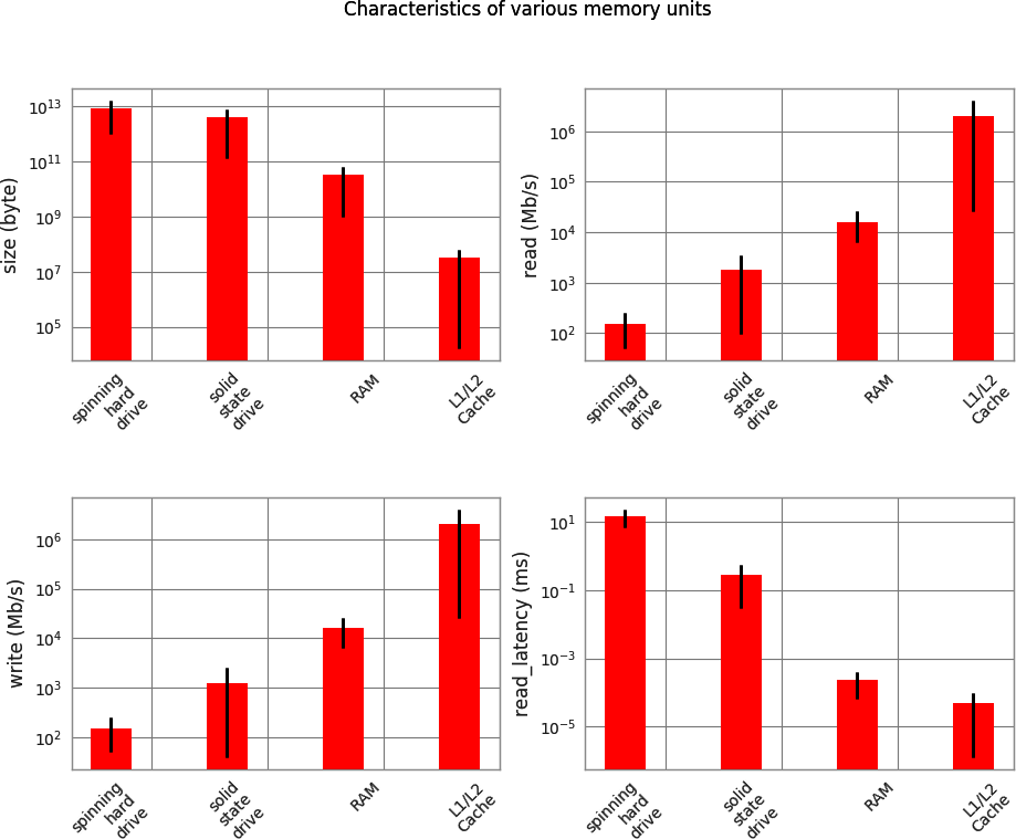
Figure 1-2. Characteristic values for different types of memory units (values from February 2014)

Communications Layers

Finally, let’s look at how all of these fundamental blocks communicate with each other. Many modes of communication exist, but all are variants on a thing called a bus.

The frontside bus, for example, is the connection between the RAM and the L1/L2 cache. It moves data that is ready to be transformed by the processor into the staging ground to get ready for calculation, and it moves finished calculations out. There are other buses, too, such as the external bus that acts as the main route from hardware devices (such as hard drives and networking cards) to the CPU and system memory. This external bus is generally slower than the frontside bus.

In fact, many of the benefits of the L1/L2 cache are attributable to the faster bus. Being able to queue up data necessary for computation in large chunks on a slow bus (from RAM to cache) and then having it available at very fast speeds from the cache lines (from cache to CPU) enables the CPU to do more calculations without waiting such a long time.

Similarly, many of the drawbacks of using a GPU come from the bus it is connected on: since the GPU is generally a peripheral device, it communicates through the PCI bus, which is much slower than the frontside bus. As a result, getting data into and out of the GPU can be quite a taxing operation. The advent of heterogeneous computing, or computing blocks that have both a CPU and a GPU on the frontside bus, aims at reducing the data transfer cost and making GPU computing more of an available option, even when a lot of data must be transferred.

In addition to the communication blocks within the computer, the network can be thought of as yet another communication block. This block, though, is much more pliable than the ones discussed previously; a network device can be connected to a memory device, such as a network attached storage (NAS) device or another computing block, as in a computing node in a cluster. However, network communications are generally much slower than the other types of communications mentioned previously. While the frontside bus can transfer dozens of gigabits per second, the network is limited to the order of several dozen megabits.

It is clear, then, that the main property of a bus is its speed: how much data it can move in a given amount of time. This property is given by combining two quantities: how much data can be moved in one transfer (bus width) and how many transfers the bus can do per second (bus frequency). It is important to note that the data moved in one transfer is always sequential: a chunk of data is read off of the memory and moved to a different place. Thus, the speed of a bus is broken into these two quantities because individually they can affect different aspects of computation: a large bus width can help vectorized code (or any code that sequentially reads through memory) by making it possible to move all the relevant data in one transfer, while, on the other hand, having a small bus width but a very high frequency of transfers can help code that must do many reads from random parts of memory. Interestingly, one of the ways that these properties are changed by computer designers is by the physical layout of the motherboard: when chips are placed close to one another, the length of the physical wires joining them is smaller, which can allow for faster transfer speeds. In addition, the number of wires itself dictates the width of the bus (giving real physical meaning to the term!).

Since interfaces can be tuned to give the right performance for a specific application, it is no surprise that there are hundreds of types. Figure 1-3 shows the bitrates for a sampling of common interfaces. Note that this doesn’t speak at all about the latency of the connections, which dictates how long it takes for a data request to be responded to (although latency is very computer-dependent, some basic limitations are inherent to the interfaces being used).

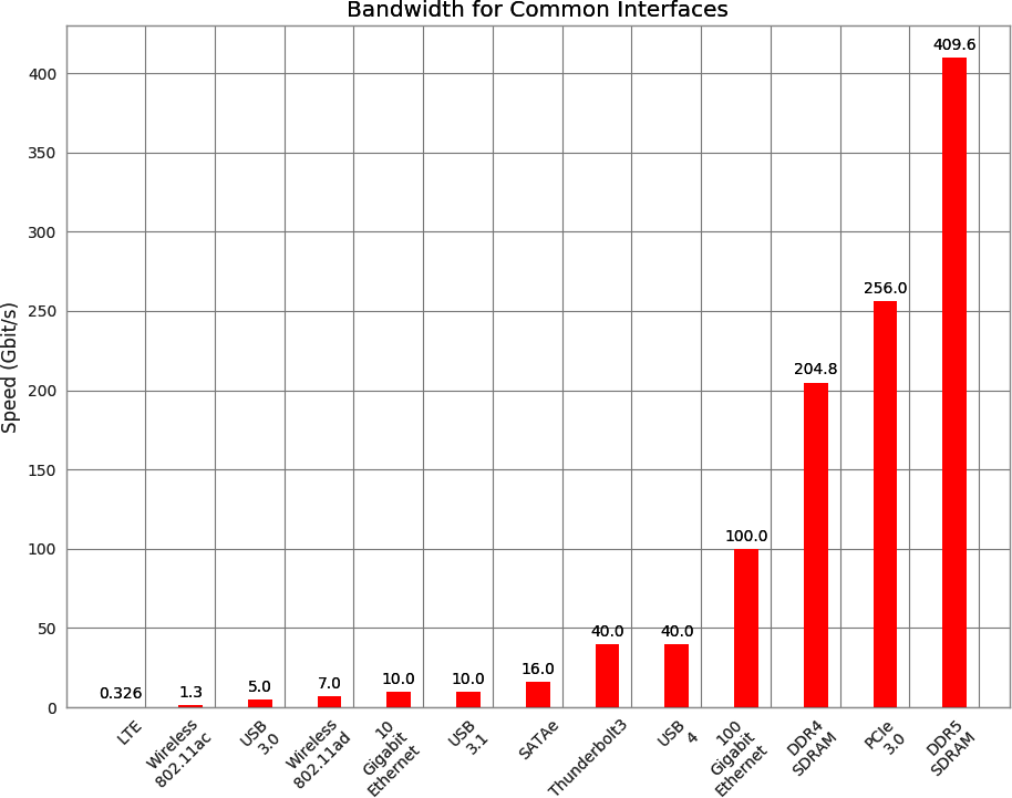
Figure 1-3. Connection speeds of various common interfaces³

Putting the Fundamental Elements Together

Understanding the basic components of a computer is not enough to fully understand the problems of high performance programming. The interplay of all of these components and how they work together to solve a problem introduces extra levels of complexity. In this section we will explore some toy problems, illustrating how the ideal solutions would work and how Python approaches them.

A warning: this section may seem bleak—most of the remarks in this section seem to say that Python is natively incapable of dealing with the problems of performance. This is untrue, for two reasons. First, among all of the “components of performant computing,” we have neglected one very important component: the developer. What native Python may lack in performance, it gets back right away with speed of development. Furthermore, throughout the book we will introduce modules and philosophies that can help mitigate many of the problems described here with relative ease. With both of these aspects combined, we will keep the fast development mindset of Python while removing many of the performance constraints.

Idealized Computing Versus the Python Virtual Machine

To better understand the components of high performance programming, let’s look at a simple code sample that checks whether a number is prime:

import math

def check_prime(number):
    sqrt_number = math.sqrt(number)
    for i in range(2, int(sqrt_number) + 1):
        if (number / i).is_integer():
            return False
    return True

print(f"check_prime(10,000,000) = {check_prime(10_000_000)}")
# check_prime(10,000,000) = False
print(f"check_prime(10,000,019) = {check_prime(10_000_019)}")
# check_prime(10,000,019) = True

Let’s analyze this code using our abstract model of computation and then draw comparisons to what happens when Python runs this code. As with any abstraction, we will neglect many of the subtleties in both the idealized computer and the way that Python runs the code. However, this is generally a good exercise to perform before solving a problem: think about the general components of the algorithm and what would be the best way for the computing components to come together to find a solution. By understanding this ideal situation and having knowledge of what is actually happening under the hood in Python, we can iteratively bring our Python code closer to the optimal code.

Idealized computing

When the code starts, we have the value of number stored in RAM. To calculate sqrt_number, we need to send the value of number to the CPU. Ideally, we could send the value once; it would get stored inside the CPU’s L1/L2 cache, and the CPU would do the calculations and then send the values back to RAM to get stored. This scenario is ideal because we have minimized the number of reads of the value of number from RAM, instead opting for reads from the L1/L2 cache, which are much faster. Furthermore, we have minimized the number of data transfers through the frontside bus, by using the L1/L2 cache which is connected directly to the CPU.

Tip

This theme of keeping data where it is needed and moving it as little as possible is very important when it comes to optimization. The concept of “heavy data” refers to the time and effort required to move data around, which is something we would like to avoid.

For the loop in the code, rather than sending one value of i at a time to the CPU, we would like to send both number and several values of i to the CPU to check at the same time. This is possible because the CPU vectorizes operations with no additional time cost, meaning it can do multiple independent computations at the same time. So we want to send number to the CPU cache, in addition to as many values of i as the cache can hold. For each of the number/i pairs, we will divide them and check if the result is a whole number; then we will send a signal back indicating whether any of the values was indeed an integer. If so, the function ends. If not, we repeat. In this way, we need to communicate back only one result for many values of i, rather than depending on the slow bus for every value. This takes advantage of a CPU’s ability to vectorize a calculation, or run one instruction on multiple data in one clock cycle.

This concept of vectorization is illustrated by the following code:

import math

def check_prime(number):
    sqrt_number = math.sqrt(number)
    numbers = range(2, int(sqrt_number)+1)
    for i in range(0, len(numbers), 5):
      # the following line is not valid Python code
        result = (number / numbers[i:(i + 5)]).is_integer()
        if any(result):
            return False
    return True

Here, we set up the processing such that the division and the checking for integers are done on a set of five values of i at a time. If properly vectorized, the CPU can do this line in one step as opposed to doing a separate calculation for every i. Ideally, the any(result) operation would also happen in the CPU without having to transfer the results back to RAM. We will talk more about vectorization, how it works, and when it benefits your code in Chapter 6.

Python’s virtual machine

The Python interpreter does a lot of work to try to abstract away the underlying computing elements that are being used. At no point does a programmer need to worry about allocating memory for arrays, how to arrange that memory, or in what sequence it is being sent to the CPU. This is a benefit of Python, since it lets you focus on the algorithms that are being implemented. However, it comes at a huge performance cost.

It is important to realize that at its core, Python is indeed running a set of very optimized instructions. The trick, however, is getting Python to perform them in the correct sequence to achieve better performance. For example, it is quite easy to see that, in the following example, search_fast will run faster than search_slow simply because it skips the unnecessary computations that result from not terminating the loop early, even though both solutions have runtime O(n). However, things can get complicated when dealing with derived types, special Python methods, or third-party modules. For example, can you immediately tell which function will be faster: search_unknown1 or search_unknown2?

def search_fast(haystack, needle):
    for item in haystack:
        if item == needle:
            return True
    return False

def search_slow(haystack, needle):
    return_value = False
    for item in haystack:
        if item == needle:
            return_value = True
    return return_value

def search_unknown1(haystack, needle):
    return any((item == needle for item in haystack))

def search_unknown2(haystack, needle):
    return any([item == needle for item in haystack])

Identifying slow regions of code through profiling and finding more efficient ways of doing the same calculations is similar to finding these useless operations and removing them; the end result is the same, but the number of computations and data transfers is reduced drastically.

One of the impacts of this abstraction layer is that vectorization is not immediately achievable. Our initial prime number routine will run one iteration of the loop per value of i instead of combining several iterations. However, looking at the abstracted vectorization example, we see that it is not valid Python code, since we cannot divide a float by a list. External libraries such as numpy will help with this situation by adding the ability to do vectorized mathematical operations.

Furthermore, Python’s abstraction hurts any optimizations that rely on keeping the L1/L2 cache filled with the relevant data for the next computation. This comes from many factors, the first being that Python objects are not laid out in the most optimal way in memory. This is a consequence of Python being a garbage-collected language—memory is automatically allocated and freed when needed. This creates memory fragmentation that can hurt the transfers to the CPU caches. In addition, at no point is there an opportunity to change the layout of a data structure directly in memory, which means that one transfer on the bus may not contain all the relevant information for a computation, even though it might have all fit within the bus width.⁴

A second, more fundamental problem comes from Python’s dynamic types and the language not being compiled. As many C programmers have learned throughout the years, the compiler is often smarter than you are. When compiling code that is static, the compiler can do many tricks to change the way things are laid out and how the CPU will run certain instructions in order to optimize them. Python, however, is not compiled: to make matters worse, it has dynamic types, which means that inferring any possible opportunities for optimizations algorithmically is drastically harder since code functionality can be changed during runtime. There are many ways to mitigate this problem, foremost being the use of Cython, which allows Python code to be compiled and allows the user to create “hints” to the compiler as to how dynamic the code actually is.

Finally, the previously mentioned GIL can hurt performance if trying to parallelize this code. For example, let’s assume we change the code to use multiple CPU cores such that each core gets a chunk of the numbers from 2 to sqrtN. Each core can do its calculation for its chunk of numbers, and then, when the calculations are all done, the cores can compare their calculations. Although we lose the early termination of the loop since each core doesn’t know if a solution has been found, we can reduce the number of checks each core has to do (if we had M cores, each core would have to do sqrtN / M checks). However, because of the GIL, only one core can be used at a time. This means that we would effectively be running the same code as the unparalleled version, but we no longer have early termination. We can avoid this problem by using multiple processes (with the multiprocessing module) instead of multiple threads, or by using Cython or foreign functions.

So Why Use Python?

Python is highly expressive and easy to learn—new programmers quickly discover that they can do quite a lot in a short space of time. Many Python libraries wrap tools written in other languages to make it easy to call other systems; for example, the scikit-learn machine learning system wraps LIBLINEAR and LIBSVM (both of which are written in C), and the numpy library includes BLAS and other C and Fortran libraries. As a result, Python code that properly utilizes these modules can indeed be as fast as comparable C code.

Python is described as “batteries included,” as many important tools and stable libraries are built in. These include the following:

unicode and bytes

Baked into the core language

array

Memory-efficient arrays for primitive types

math

Basic mathematical operations, including some simple statistics

sqlite3

A wrapper around the prevalent SQL file-based storage engine SQLite3

collections

A wide variety of objects, including a deque, counter, and dictionary variants

asyncio

Concurrent support for I/O-bound tasks using async and await syntax

A huge variety of libraries can be found outside the core language, including these:

numpy

A numerical Python library (a bedrock library for anything to do with matrices)

scipy

A very large collection of trusted scientific libraries, often wrapping highly respected C and Fortran libraries

pandas

A library for data analysis, similar to R’s data frames or an Excel spreadsheet, built on scipy and numpy

scikit-learn

Rapidly turning into the default machine learning library, built on scipy

tornado

A library that provides easy bindings for concurrency

PyTorch and TensorFlow

Deep learning frameworks from Facebook and Google with strong Python and GPU support

NLTK, SpaCy, and Gensim

Natural language-processing libraries with deep Python support

Database bindings

For communicating with virtually all databases, including Redis, MongoDB, HDF5, and SQL

Web development frameworks

Performant systems for creating websites, such as aiohttp, django, pyramid, flask, and tornado

OpenCV

Bindings for computer vision

API bindings

For easy access to popular web APIs such as Google, Twitter, and LinkedIn

A large selection of managed environments and shells is available to fit various deployment scenarios, including the following:

• The standard distribution, available at http://python.org

• pipenv, pyenv, and virtualenv for simple, lightweight, and portable Python environments

• Docker for simple-to-start-and-reproduce environments for development or production

• Anaconda Inc.’s Anaconda, a scientifically focused environment

• Sage, a Matlab-like environment that includes an integrated development environment (IDE)

• IPython, an interactive Python shell heavily used by scientists and developers

• Jupyter Notebook, a browser-based extension to IPython, heavily used for teaching and demonstrations

One of Python’s main strengths is that it enables fast prototyping of an idea. Because of the wide variety of supporting libraries, it is easy to test whether an idea is feasible, even if the first implementation might be rather flaky.

If you want to make your mathematical routines faster, look to numpy. If you want to experiment with machine learning, try scikit-learn. If you are cleaning and manipulating data, then pandas is a good choice.

In general, it is sensible to raise the question, “If our system runs faster, will we as a team run slower in the long run?” It is always possible to squeeze more performance out of a system if enough work-hours are invested, but this might lead to brittle and poorly understood optimizations that ultimately trip up the team.

One example might be the introduction of Cython (see “Cython”), a compiler-based approach to annotating Python code with C-like types so the transformed code can be compiled using a C compiler. While the speed gains can be impressive (often achieving C-like speeds with relatively little effort), the cost of supporting this code will increase. In particular, it might be harder to support this new module, as team members will need a certain maturity in their programming ability to understand some of the trade-offs that have occurred when leaving the Python virtual machine that introduced the performance increase.

How to Be a Highly Performant Programmer

Writing high performance code is only one part of being highly performant with successful projects over the longer term. Overall team velocity is far more important than speedups and complicated solutions. Several factors are key to this—good structure, documentation, debuggability, and shared standards.

Let’s say you create a prototype. You didn’t test it thoroughly, and it didn’t get reviewed by your team. It does seem to be “good enough,” and it gets pushed to production. Since it was never written in a structured way, it lacks tests and is undocumented. All of a sudden there’s an inertia-causing piece of code for someone else to support, and often management can’t quantify the cost to the team.

As this solution is hard to maintain, it tends to stay unloved—it never gets restructured, it doesn’t get the tests that’d help the team refactor it, and nobody else likes to touch it, so it falls to one developer to keep it running. This can cause an awful bottleneck at times of stress and raises a significant risk: what would happen if that developer left the project?

Typically, this development style occurs when the management team doesn’t understand the ongoing inertia that’s caused by hard-to-maintain code. Demonstrating that in the longer-term tests and documentation can help a team stay highly productive and can help convince managers to allocate time to “cleaning up” this prototype code.

In a research environment, it is common to create many Jupyter Notebooks using poor coding practices while iterating through ideas and different datasets. The intention is always to “write it up properly” at a later stage, but that later stage never occurs. In the end, a working result is obtained, but the infrastructure to reproduce it, test it, and trust the result is missing. Once again the risk factors are high, and the trust in the result will be low.

There’s a general approach that will serve you well:

Make it work

First you build a good-enough solution. It is very sensible to “build one to throw away” that acts as a prototype solution, enabling a better structure to be used for the second version. It is always sensible to do some up-front planning before coding; otherwise, you’ll come to reflect that “We saved an hour’s thinking by coding all afternoon.” In some fields this is better known as “Measure twice, cut once.”

Make it right

Next, you add a strong test suite backed by documentation and clear reproducibility instructions so that another team member can take it on.

Make it fast

Finally, we can focus on profiling and compiling or parallelization and using the existing test suite to confirm that the new, faster solution still works as expected.

Good Working Practices

There are a few “must haves”—documentation, good structure, and testing are key.

Some project-level documentation will help you stick to a clean structure. It’ll also help you and your colleagues in the future. Nobody will thank you (yourself included) if you skip this part. Writing this up in a README file at the top level is a sensible starting point; it can always be expanded into a docs/ folder later if required.

Explain the purpose of the project, what’s in the folders, where the data comes from, which files are critical, and how to run it all, including how to run the tests.

Micha recommends also using Docker. A top-level Dockerfile will explain to your future-self exactly which libraries you need from the operating system to make this project run successfully. It also removes the difficulty of running this code on other machines or deploying it to a cloud environment.

Add a tests/ folder and add some unit tests. We prefer pytest as a modern test runner, as it builds on Python’s built-in unittest module. Start with just a couple of tests and then build them up. Progress to using the coverage tool, which will report how many lines of your code are actually covered by the tests—it’ll help avoid nasty surprises.

If you’re inheriting legacy code and it lacks tests, a high-value activity is to add some tests up front. Some “integration tests” that check the overall flow of the project and confirm that with certain input data you get specific output results will help your sanity as you subsequently make modifications.

Every time something in the code bites you, add a test. There’s no value to being bitten twice by the same problem.

Docstrings in your code for each function, class, and module will always help you. Aim to provide a useful description of what’s achieved by the function, and where possible include a short example to demonstrate the expected output. Look at the docstrings inside numpy and scikit-learn if you’d like inspiration.

Whenever your code becomes too long—such as functions longer than one screen—be comfortable with refactoring the code to make it shorter. Shorter code is easier to test and easier to support.

Tip

When you’re developing your tests, think about following a test-driven development methodology. When you know exactly what you need to develop and you have testable examples at hand—this method becomes very efficient.

You write your tests, run them, watch them fail, and then add the functions and the necessary minimum logic to support the tests that you’ve written. When your tests all work, you’re done. By figuring out the expected input and output of a function ahead of time, you’ll find implementing the logic of the function relatively straightforward.

If you can’t define your tests ahead of time, it naturally raises the question, do you really understand what your function needs to do? If not, can you write it correctly in an efficient manner? This method doesn’t work so well if you’re in a creative process and researching data that you don’t yet understand well.

Always use source control—you’ll only thank yourself when you overwrite something critical at an inconvenient moment. Get used to committing frequently (daily, or even every 10 minutes) and pushing to your repository every day.

Keep to the standard PEP8 coding standard. Even better, adopt black (the opinionated code formatter) on a pre-commit source control hook so it just rewrites your code to the standard for you. Use flake8 to lint your code to avoid other mistakes.

Creating environments that are isolated from the operating system will make your life easier. Ian prefers Anaconda, while Micha prefers pipenv coupled with Docker. Both are sensible solutions and are significantly better than using the operating system’s global Python environment!

Remember that automation is your friend. Doing less manual work means there’s less chance of errors creeping in. Automated build systems, continuous integration with automated test suite runners, and automated deployment systems turn tedious and error-prone tasks into standard processes that anyone can run and support.

Finally, remember that readability is far more important than being clever. Short snippets of complex and hard-to-read code will be hard for you and your colleagues to maintain, so people will be scared of touching this code. Instead, write a longer, easier-to-read function and back it with useful documentation showing what it’ll return, and complement this with tests to confirm that it does work as you expect.

Some Thoughts on Good Notebook Practice

If you’re using Jupyter Notebooks, they’re great for visual communication, but they facilitate laziness. If you find yourself leaving long functions inside your Notebooks, be comfortable extracting them out to a Python module and then adding tests.

Consider prototyping your code in IPython or the QTConsole; turn lines of code into functions in a Notebook and then promote them out of the Notebook and into a module complemented by tests. Finally, consider wrapping the code in a class if encapsulation and data hiding are useful.

Liberally spread assert statements throughout a Notebook to check that your functions are behaving as expected. You can’t easily test code inside a Notebook, and until you’ve refactored your functions into separate modules, assert checks are a simple way to add some level of validation. You shouldn’t trust this code until you’ve extracted it to a module and written sensible unit tests.

Using assert statements to check data in your code should be frowned upon. It is an easy way to assert that certain conditions are being met, but it isn’t idiomatic Python. To make your code easier to read by other developers, check your expected data state and then raise an appropriate exception if the check fails. A common exception would be ValueError if a function encounters an unexpected value. The Bulwark library is an example of a testing framework focused on Pandas to check that your data meets the specified constraints.

You may also want to add some sanity checks at the end of your Notebook—a mixture of logic checks and raise and print statements that demonstrate that you’ve just generated exactly what you needed. When you return to this code in six months, you’ll thank yourself for making it easy to see that it worked correctly all the way through!

One difficulty with Notebooks is sharing code with source control systems. nbdime is one of a growing set of new tools that let you diff your Notebooks. It is a lifesaver and enables collaboration with colleagues.

Getting the Joy Back into Your Work

Life can be complicated. In the five years since your authors wrote the first edition of this book, we’ve jointly experienced through friends and family a number of life situations, including depression, cancer, home relocations, successful business exits and failures, and career direction shifts. Inevitably, these external events will have an impact on anyone’s work and outlook on life.

Remember to keep looking for the joy in new activities. There are always interesting details or requirements once you start poking around. You might ask, “why did they make that decision?” and “how would I do it differently?” and all of a sudden you’re ready to start a conversation about how things might be changed or improved.

Keep a log of things that are worth celebrating. It is so easy to forget about accomplishments and to get caught up in the day-to-day. People get burned out because they’re always running to keep up, and they forget how much progress they’ve made.

We suggest that you build a list of items worth celebrating and note how you celebrate them. Ian keeps such a list—he’s happily surprised when he goes to update the list and sees just how many cool things have happened (and might otherwise have been forgotten!) in the last year. These shouldn’t just be work milestones; include hobbies and sports, and celebrate the milestones you’ve achieved. Micha makes sure to prioritize her personal life and spend days away from the computer to work on nontechnical projects. It is critical to keep developing your skill set, but it is not necessary to burn out!

Programming, particularly when performance focused, thrives on a sense of curiosity and a willingness to always delve deeper into the technical details. Unfortunately, this curiosity is the first thing to go when you burn out; so take your time and make sure you enjoy the journey, and keep the joy and the curiosity.

¹ Not to be confused with interprocess communication, which shares the same acronym—we’ll look at that topic in Chapter 9.

² Speeds in this section are from https://oreil.ly/pToi7.

³ Data is from https://oreil.ly/7SC8d.

⁴ In Chapter 6, we’ll see how we can regain this control and tune our code all the way down to the memory utilization patterns.