Chapter 4. Representing Data and Engineering Features
So far, we’ve assumed that our data comes in as a two-dimensional array of floating-point numbers, where each column is a continuous feature that describes the data points. For many applications, this is not how the data is collected. A particularly common type of feature is the categorical features. Also known as discrete features, these are usually not numeric. The distinction between categorical features and continuous features is analogous to the distinction between classification and regression, only on the input side rather than the output side. Examples of continuous features that we have seen are pixel brightnesses and size measurements of plant flowers. Examples of categorical features are the brand of a product, the color of a product, or the department (books, clothing, hardware) it is sold in. These are all properties that can describe a product, but they don’t vary in a continuous way. A product belongs either in the clothing department or in the books department. There is no middle ground between books and clothing, and no natural order for the different categories (books is not greater or less than clothing, hardware is not between books and clothing, etc.).
Regardless of the types of features your data consists of, how you represent them can have an enormous effect on the performance of machine learning models. We saw in Chapters 2 and 3 that scaling of the data is important. In other words, if you don’t rescale your data (say, to unit variance), then it makes a difference whether you represent a measurement in centimeters or inches. We also saw in Chapter 2 that it can be helpful to augment your data with additional features, like adding interactions (products) of features or more general polynomials.
The question of how to represent your data best for a particular application is known as feature engineering, and it is one of the main tasks of data scientists and machine learning practitioners trying to solve real-world problems. Representing your data in the right way can have a bigger influence on the performance of a supervised model than the exact parameters you choose.
In this chapter, we will first go over the important and very common case of categorical features, and then give some examples of helpful transformations for specific combinations of features and models.
4.1 Categorical Variables
As an example, we will use the dataset of adult incomes in the United
States, derived from the 1994 census database. The task of the adult
dataset is to predict whether a worker has an income of over $50,000 or
under $50,000. The features in this dataset include the workers’ ages, how
they are employed (self employed, private industry employee, government
employee, etc.), their education, their gender, their working hours per
week, occupation, and more. Table 4-1 shows the first few
entries in the dataset.
| age | workclass | education | gender | hours-per-week | occupation | income | |
|---|---|---|---|---|---|---|---|
0 |
39 |
State-gov |
Bachelors |
Male |
40 |
Adm-clerical |
<=50K |
1 |
50 |
Self-emp-not-inc |
Bachelors |
Male |
13 |
Exec-managerial |
<=50K |
2 |
38 |
Private |
HS-grad |
Male |
40 |
Handlers-cleaners |
<=50K |
3 |
53 |
Private |
11th |
Male |
40 |
Handlers-cleaners |
<=50K |
4 |
28 |
Private |
Bachelors |
Female |
40 |
Prof-specialty |
<=50K |
5 |
37 |
Private |
Masters |
Female |
40 |
Exec-managerial |
<=50K |
6 |
49 |
Private |
9th |
Female |
16 |
Other-service |
<=50K |
7 |
52 |
Self-emp-not-inc |
HS-grad |
Male |
45 |
Exec-managerial |
>50K |
8 |
31 |
Private |
Masters |
Female |
50 |
Prof-specialty |
>50K |
9 |
42 |
Private |
Bachelors |
Male |
40 |
Exec-managerial |
>50K |
10 |
37 |
Private |
Some-college |
Male |
80 |
Exec-managerial |
>50K |
The task is phrased as a classification task with the two classes being
income <=50k and >50k. It would also be possible to predict the
exact income, and make this a regression task. However, that would be
much more difficult, and the 50K division is interesting to understand
on its own.
In this dataset, age and hours-per-week are continuous features,
which we know how to treat. The workclass, education, sex, and
occupation features are categorical, however. All of them come from a
fixed list of possible values, as opposed to a range, and denote a
qualitative property, as opposed to a quantity.
As a starting point, let’s say we want to learn a logistic regression classifier on this data. We know from Chapter 2 that a logistic regression makes predictions, ŷ, using the following formula:
- ŷ = w[0] * x[0] + w[1] * x[1] + ... + w[p] * x[p] + b > 0
where w[i] and b are coefficients learned from the training set and
x[i] are the input features. This formula makes sense when x[i] are
numbers, but not when x[2] is "Masters" or "Bachelors". Clearly we
need to represent our data in some different way when applying logistic
regression. The next section will explain how we can overcome this
problem.
4.1.1 One-Hot-Encoding (Dummy Variables)
By far the most common way to represent categorical variables is using
the one-hot-encoding or one-out-of-N encoding, also known as dummy
variables. The idea behind dummy variables is to replace a categorical
variable with one or more new features that can have the values 0 and 1.
The values 0 and 1 make sense in the formula for linear binary
classification (and for all other models in scikit-learn), and we can
represent any number of categories by introducing one new feature per
category, as described here.
Let’s say for the workclass feature we have
possible values of "Government Employee", "Private Employee",
"Self Employed", and "Self Employed Incorporated". To encode these
four possible values, we create four new features, called
"Government Employee", "Private Employee", "Self Employed", and
"Self Employed Incorporated". A feature is 1 if workclass for this
person has the corresponding value and 0 otherwise, so exactly one of
the four new features will be 1 for each data point. This is why this is
called one-hot or one-out-of-N encoding.
The principle is illustrated in Table 4-2. A single feature is
encoded using four new features. When using this data in a machine
learning algorithm, we would drop the original workclass feature and
only keep the 0–1 features.
| workclass | Government Employee | Private Employee | Self Employed | Self Employed Incorporated |
|---|---|---|---|---|
Government Employee |
1 |
0 |
0 |
0 |
Private Employee |
0 |
1 |
0 |
0 |
Self Employed |
0 |
0 |
1 |
0 |
Self Employed Incorporated |
0 |
0 |
0 |
1 |
Note
The one-hot encoding we use is quite similar, but not identical, to the dummy coding used in statistics. For simplicity, we encode each category with a different binary feature. In statistics, it is common to encode a categorical feature with k different possible values into k–1 features (the last one is represented as all zeros). This is done to simplify the analysis (more technically, this will avoid making the data matrix rank-deficient).
There are two ways to convert your data to a one-hot encoding of
categorical variables, using either pandas or scikit-learn. Let’s
see how we can do it using pandas. We start by loading the data using pandas from a comma-separated values (CSV) file:
In[1]:
importos# The file has no headers naming the columns, so we pass header=None# and provide the column names explicitly in "names"adult_path=os.path.join(mglearn.datasets.DATA_PATH,"adult.data")data=pd.read_csv(adult_path,header=None,index_col=False,names=['age','workclass','fnlwgt','education','education-num','marital-status','occupation','relationship','race','gender','capital-gain','capital-loss','hours-per-week','native-country','income'])# For illustration purposes, we only select some of the columnsdata=data[['age','workclass','education','gender','hours-per-week','occupation','income']]# IPython.display allows nice output formatting within the Jupyter notebookdisplay(data.head())
Table 4-3 shows the result.
| age | workclass | education | gender | hours-per-week | occupation | income | |
|---|---|---|---|---|---|---|---|
0 |
39 |
State-gov |
Bachelors |
Male |
40 |
Adm-clerical |
<=50K |
1 |
50 |
Self-emp-not-inc |
Bachelors |
Male |
13 |
Exec-managerial |
<=50K |
2 |
38 |
Private |
HS-grad |
Male |
40 |
Handlers-cleaners |
<=50K |
3 |
53 |
Private |
11th |
Male |
40 |
Handlers-cleaners |
<=50K |
4 |
28 |
Private |
Bachelors |
Female |
40 |
Prof-specialty |
<=50K |
Checking string-encoded categorical data
After reading a dataset like this, it is often good to first check if a
column actually contains meaningful categorical data. When working with
data that was input by humans (say, users on a website), there might not
be a fixed set of categories, and differences in spelling and
capitalization might require preprocessing. For example, it might be
that some people specified gender as “male” and some as “man,” and we
might want to represent these two inputs using the same category. A good
way to check the contents of a column is using the value_counts
method of a pandas Series (the type of a single column in a
DataFrame), to show us what the unique values are and how often they
appear:
In[2]:
(data.gender.value_counts())
Out[2]:
 Male      21790
 Female    10771
Name: gender, dtype: int64
We can see that there are exactly two values for gender in this
dataset, Male and Female, meaning the data is already in a good
format to be represented using one-hot-encoding. In a real application,
you should look at all columns and check their values. We will skip
this here for brevity’s sake.
There is a very simple way to encode the data in pandas, using the
get_dummies function. The get_dummies function automatically
transforms all columns that have object type (like strings) or are
categorical (which is a special pandas concept that we haven’t talked
about yet):
In[3]:
("Original features:\n",list(data.columns),"\n")data_dummies=pd.get_dummies(data)("Features after get_dummies:\n",list(data_dummies.columns))
Out[3]:
Original features:
 ['age', 'workclass', 'education', 'gender', 'hours-per-week', 'occupation',
  'income']

Features after get_dummies:
 ['age', 'hours-per-week', 'workclass_ ?', 'workclass_ Federal-gov',
  'workclass_ Local-gov', 'workclass_ Never-worked', 'workclass_ Private',
  'workclass_ Self-emp-inc', 'workclass_ Self-emp-not-inc',
  'workclass_ State-gov', 'workclass_ Without-pay', 'education_ 10th',
  'education_ 11th', 'education_ 12th', 'education_ 1st-4th',
   ...
  'education_ Preschool', 'education_ Prof-school', 'education_ Some-college',
  'gender_ Female', 'gender_ Male', 'occupation_ ?',
  'occupation_ Adm-clerical', 'occupation_ Armed-Forces',
  'occupation_ Craft-repair', 'occupation_ Exec-managerial',
  'occupation_ Farming-fishing', 'occupation_ Handlers-cleaners',
  ...
  'occupation_ Tech-support', 'occupation_ Transport-moving',
  'income_ <=50K', 'income_ >50K']
You can see that the continuous features age and hours-per-week were
not touched, while the categorical features were expanded into one new
feature for each possible value:
In[4]:
data_dummies.head()
Out[4]:
| age | hours-per-week | workclass_ ? | workclass_ Federal-gov | workclass_ Local-gov | … | occupation_ Tech-support | occupation_ Transport-moving | income_ <=50K | income_ >50K | |
|---|---|---|---|---|---|---|---|---|---|---|
0 |
39 |
40 |
0.0 |
0.0 |
0.0 |
… |
0.0 |
0.0 |
1.0 |
0.0 |
1 |
50 |
13 |
0.0 |
0.0 |
0.0 |
… |
0.0 |
0.0 |
1.0 |
0.0 |
2 |
38 |
40 |
0.0 |
0.0 |
0.0 |
… |
0.0 |
0.0 |
1.0 |
0.0 |
3 |
53 |
40 |
0.0 |
0.0 |
0.0 |
… |
0.0 |
0.0 |
1.0 |
0.0 |
4 |
28 |
40 |
0.0 |
0.0 |
0.0 |
… |
0.0 |
0.0 |
1.0 |
0.0 |
5 rows × 46 columns
We can now use the values attribute to convert the data_dummies
DataFrame into a NumPy array, and then train a machine learning model on
it. Be careful to separate the target variable (which is now encoded in
two income columns) from the data before training a model. Including
the output variable, or some derived property of the output variable,
into the feature representation is a very common mistake in building
supervised machine learning models.
Warning
Be careful: column indexing in pandas includes the end of the
range, so 'age':'occupation_ Transport-moving' is inclusive of
occupation_ Transport-moving. This is different from slicing a NumPy
array, where the end of a range is not included: for example,
np.arange(11)[0:10] doesn’t include the entry with index 10.
In this case, we extract only the columns containing features—that is, all columns from age to occupation_ Transport-moving. This range contains all the features but not the target:
In[5]:
features=data_dummies.loc[:,'age':'occupation_ Transport-moving']# Extract NumPy arraysX=features.valuesy=data_dummies['income_ >50K'].values("X.shape: {} y.shape: {}".format(X.shape,y.shape))
Out[5]:
X.shape: (32561, 44) y.shape: (32561,)
Now the data is represented in a way that scikit-learn can work with,
and we can proceed as usual:
In[6]:
fromsklearn.linear_modelimportLogisticRegressionfromsklearn.model_selectionimporttrain_test_splitX_train,X_test,y_train,y_test=train_test_split(X,y,random_state=0)logreg=LogisticRegression()logreg.fit(X_train,y_train)("Test score: {:.2f}".format(logreg.score(X_test,y_test)))
Out[6]:
Test score: 0.81
Warning
In this example, we called get_dummies on a DataFrame
containing both the training and the test data. This is important to
ensure categorical values are represented in the same way in the
training set and the test set.
Imagine we have the training and test sets in two different
DataFrames. If the "Private Employee" value for the workclass feature
does not appear in the test set, pandas will assume there are only
three possible values for this feature and will create only three new
dummy features. Now our training and test sets have different numbers of
features, and we can’t apply the model we learned on the training set to
the test set anymore. Even worse, imagine the workclass feature has
the values "Government Employee" and "Private Employee" in the training
set, and "Self Employed" and "Self Employed Incorporated" in the test
set. In both cases, pandas will create two new dummy features, so the
encoded DataFrames will have the same number of features. However, the
two dummy features have entirely different meanings in the training and
test sets. The column that means "Government Employee" for the
training set would encode "Self Employed" for the test set.
If we built a machine learning model on this data it would work very
badly, because it would assume the columns mean the same things (because they are in
the same position) when in fact they mean very different things. To fix this,
either call get_dummies on a DataFrame that contains both the training and
the test data points, or make sure that the column names are the same
for the training and test sets after calling get_dummies, to ensure they
have the same semantics.
4.1.2 Numbers Can Encode Categoricals
In the example of the adult dataset, the categorical variables were
encoded as strings. On the one hand, that opens up the possibility of
spelling errors, but on the other hand, it clearly marks a variable as
categorical. Often, whether for ease of storage or because of the way
the data is collected, categorical variables are encoded as integers.
For example, imagine the census data in the adult dataset was
collected using a questionnaire, and the answers for workclass were
recorded as 0 (first box ticked), 1 (second box ticked), 2 (third box
ticked), and so on. Now the column will contain numbers from 0 to 8,
instead of strings like "Private", and it won’t be immediately obvious to someone looking at the table representing
the dataset whether they should treat
this variable as continuous or categorical. Knowing that the numbers
indicate employment status, however, it is clear that these are very distinct
states and should not be modeled by a single continuous variable.
Warning
Categorical features are often encoded using integers.
That they are numbers doesn’t mean that they should necessarily be treated as
continuous features. It is not always clear whether an integer feature
should be treated as continuous or discrete (and one-hot-encoded). If
there is no ordering between the semantics that are encoded (like in the
workclass example), the feature must be treated as discrete. For
other cases, like five-star ratings, the better encoding depends on the
particular task and data and which machine learning algorithm is
used.
The get_dummies function in pandas treats all numbers as continuous
and will not create dummy variables for them. To illustrate, let’s
create a DataFrame object with two columns corresponding to two
different categorical features, one represented as a string and one
as an integer.
In[7]:
# create a DataFrame with an integer feature and a categorical string featuredemo_df=pd.DataFrame({'Integer Feature':[0,1,2,1],'Categorical Feature':['socks','fox','socks','box']})display(demo_df)
Table 4-4 shows the result.
| Categorical Feature | Integer Feature | |
|---|---|---|
0 |
socks |
0 |
1 |
fox |
1 |
2 |
socks |
2 |
3 |
box |
1 |
Using get_dummies will only encode the string feature and will not change
the integer feature, as you can see in Table 4-5:
In[8]:
display(pd.get_dummies(demo_df))
| Integer Feature | Categorical Feature_box | Categorical Feature_fox | Categorical Feature_socks | |
|---|---|---|---|---|
0 |
0 |
0.0 |
0.0 |
1.0 |
1 |
1 |
0.0 |
1.0 |
0.0 |
2 |
2 |
0.0 |
0.0 |
1.0 |
3 |
1 |
1.0 |
0.0 |
0.0 |
If you want dummy variables to be created for the “Integer Feature”
column, you can explicitly list the columns you want to encode using the
columns parameter. Then, both features will be treated as categorical (see Table 4-6):
In[9]:
demo_df['Integer Feature']=demo_df['Integer Feature'].astype(str)display(pd.get_dummies(demo_df,columns=['Integer Feature','Categorical Feature']))
| Integer Feature_0 | Integer Feature_1 | Integer Feature_2 | Categorical Feature_box | Categorical Feature_fox | Categorical Feature_socks | |
|---|---|---|---|---|---|---|
0 |
1.0 |
0.0 |
0.0 |
0.0 |
0.0 |
1.0 |
1 |
0.0 |
1.0 |
0.0 |
0.0 |
1.0 |
0.0 |
2 |
0.0 |
0.0 |
1.0 |
0.0 |
0.0 |
1.0 |
3 |
0.0 |
1.0 |
0.0 |
1.0 |
0.0 |
0.0 |
4.2 OneHotEncoder and ColumnTransformer: Categorical Variables with scikit-learn
As mentioned before, scikit-learn can also perform one-hot-encoding.
Using scikit-learn has the advantage of making it easy to treat
training and test set in a consistent way. One-hot-encoding is
implemented in the OneHotEncoder class1 Notably, the OneHotEncoder applies the
encoding to all input columns:
In[10]:
fromsklearn.preprocessingimportOneHotEncoder# Setting sparse=False means OneHotEncode will return a numpy array,# not a sparse matrixohe=OneHotEncoder(sparse=False)(ohe.fit_transform(demo_df))
Out[10]:
[[1. 0. 0. 0. 0. 1.]
 [0. 1. 0. 0. 1. 0.]
 [0. 0. 1. 0. 0. 1.]
 [0. 1. 0. 1. 0. 0.]]
You can see that both the string and integer feature were transformed.
As usual for scikit-learn, the output is not a DataFrame, so there
are no column names. To obtain the correspondence of the transformed
features to the original categorical variables, we can use the
get_feature_names method:
In[11]:
(ohe.get_feature_names())
Out[11]:
['x0_0' 'x0_1' 'x0_2' 'x1_box' 'x1_fox' 'x1_socks']
There, the first three columns correspond to the values 0, 1, and 2 of
the first original feature (called x0 here), while the last three
columns correspond to the values box, fox, and socks for the second
original feature (called x1 here).
In most applications, some features are categorical and some are
continuous, so OneHotEncoder is not directly applicable, as it assumes
all features are categorical. This is where the ColumnTransformer
class comes in handy: it allows you to apply different transformations to
different columns in the input data. This is incredibly useful, since
continuous and categorical features need very different kinds of
preprocessing.
Let’s go back to the example of the adult census data we considered earlier:
In[12]:
display(data.head())
Out[12]:
[cols=",,,,,,,",options="header",]
|=======================================================================
| |age |workclass |education |gender |hours-per-week |occupation |income
|0 |39 |State-gov |Bachelors |Male |40 |Adm-clerical |<=50K
|1 |50 |Self-emp-not-inc |Bachelors |Male |13 |Exec-managerial |<=50K
|2 |38 |Private |HS-grad |Male |40 |Handlers-cleaners |<=50K
|3 |53 |Private |11th |Male |40 |Handlers-cleaners |<=50K
|4 |28 |Private |Bachelors |Female |40 |Prof-specialty |<=50K
|=======================================================================
To apply, say, a linear model to this dataset to predict income, in
addition to applying one-hot-encoding to the categorical variables, we
might also want to scale the continuous variables age and
hours-per-week. This is exactly what ColumnTransformer can do for
us. Each transformation in the column transformer is specified by a name
(we will see later why this is useful), a transformer object, and the
columns this transformer should be applied to. The columns can be
specified using column names, integer indices, or boolean masks. Each
transformer is applied to the corresponding columns, and the result of
the transformations are concatenated (horizontally). For the example
earlier, using column names the specification looks like this:
In[13]:
fromsklearn.composeimportColumnTransformerfromsklearn.preprocessingimportStandardScalerct=ColumnTransformer([("scaling",StandardScaler(),['age','hours-per-week']),("onehot",OneHotEncoder(sparse=False),['workclass','education','gender','occupation'])])
Now we can use the ColumnTransformer object as we would any other
scikit-learn transformation, using fit and transform. So let’s
build a linear model as before, but this time include scaling of the
continuous variables. Note that we are calling train_test_split on the
DataFrame containing the features, not on a NumPy array. We need to
preserve the column names so that they can be used in the
ColumnTransformer.
In[14]:
fromsklearn.linear_modelimportLogisticRegressionfromsklearn.model_selectionimporttrain_test_split# get all columns apart from income for the featuresdata_features=data.drop("income",axis=1)# split dataframe and incomeX_train,X_test,y_train,y_test=train_test_split(data_features,data.income,random_state=0)ct.fit(X_train)X_train_trans=ct.transform(X_train)(X_train_trans.shape)
Out[14]:
(24420, 44)
You can see that we obtained 44 features, the same as when we used
pd.get_dummies before, except that we also scaled the continuous
features. Now we can build a LogisticRegression model:
In[15]:
logreg=LogisticRegression()logreg.fit(X_train_trans,y_train)X_test_trans=ct.transform(X_test)("Test score: {:.2f}".format(logreg.score(X_test_trans,y_test)))
Out[15]:
Test score: 0.81
In this case, scaling the data didn’t make a difference, but
encapsulating all of the preprocessing inside a transformer has
additional benefits that we will discuss later. You can access the steps
inside the ColumnTransformer via the named_transformers_ attribute:
In[16]:
ct.named_transformers_.onehot
Out[16]:
OneHotEncoder(categorical_features=None, categories=None,
       dtype=<class 'numpy.float64'>, handle_unknown='error',
       n_values=None, sparse=False)
4.3 Convenient ColumnTransformer creation with make_columntransformer
Creating a ColumnTransformer using the syntax described earlier is
sometimes a bit cumbersome, and we often don’t need user-specified names
for each step. There is a convenience function (make_columntransformer)
that will create a ColumnTranformer for us and automatically name each
step based on its class. The syntax for make_columntransformer is as
follows:
In[17]:
fromsklearn.composeimportmake_column_transformerct=make_column_transformer((['age','hours-per-week'],StandardScaler()),(['workclass','education','gender','occupation'],OneHotEncoder(sparse=False)))
A disadavantage of using the ColumnTransformer is that in version 0.20
it is not yet possible to readily find which input columns correspond to
which output columns of the column transformer in all cases.
4.4 Binning, Discretization, Linear Models, and Trees
The best way to represent data depends not only on the semantics of the
data, but also on the kind of model you are using. Linear models and
tree-based models (such as decision trees, gradient boosted trees, and
random forests), two large and very commonly used families, have very
different properties when it comes to how they work with different
feature representations. Let’s go back to the wave regression dataset
that we used in Chapter 2. It has only a single input feature. Here is a
comparison of a linear regression model and a decision tree regressor on
this dataset (see Figure 4-1):
In[18]:
fromsklearn.linear_modelimportLinearRegressionfromsklearn.treeimportDecisionTreeRegressorX,y=mglearn.datasets.make_wave(n_samples=120)line=np.linspace(-3,3,1000,endpoint=False).reshape(-1,1)reg=DecisionTreeRegressor(min_samples_leaf=3).fit(X,y)plt.plot(line,reg.predict(line),label="decision tree")reg=LinearRegression().fit(X,y)plt.plot(line,reg.predict(line),label="linear regression")plt.plot(X[:,0],y,'o',c='k')plt.ylabel("Regression output")plt.xlabel("Input feature")plt.legend(loc="best")
As you know, linear models can only model linear relationships, which are lines in the case of a single feature. The decision tree can build a much more complex model of the data. However, this is strongly dependent on the representation of the data. One way to make linear models more powerful on continuous data is to use binning (also known as discretization) of the feature to split it up into multiple features, as described here.
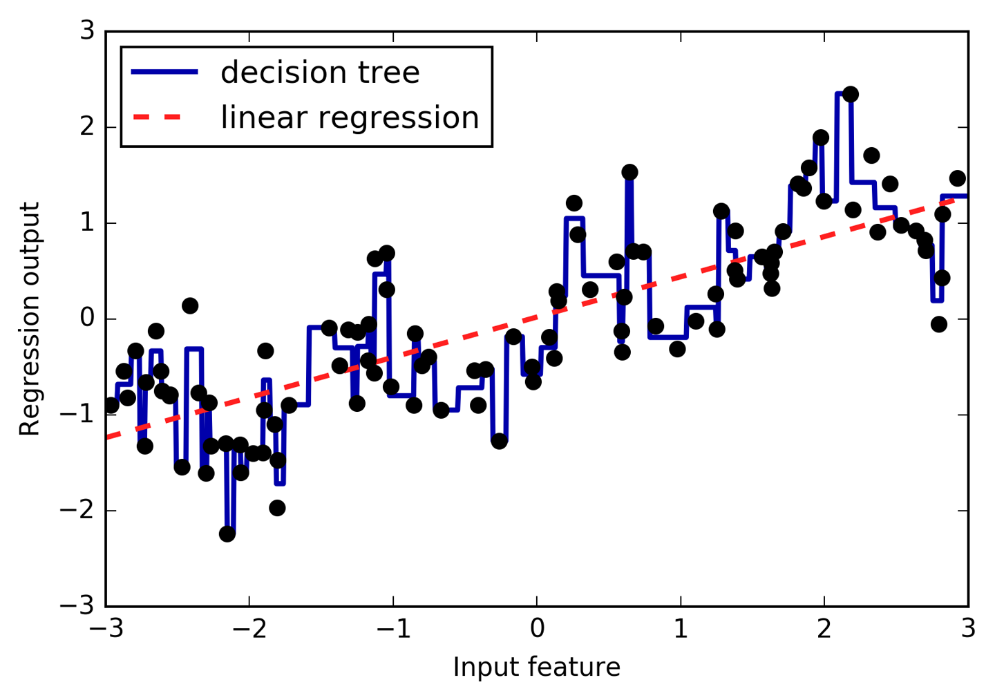
Figure 4-1. Comparing linear regression and a decision tree on the wave dataset
We imagine a partition of the input range for the feature (in this case,
the numbers from –3 to 3) into a fixed number of bins—say, 10. A data
point will then be represented by which bin it falls into. There are
several ways to define the edges of the bins; for example, giving them
uniform width (making the bin edges equidistant) or using quantiles of
the data (i.e., having smaller bins where there’s more data). Both of
these strategies are implemented in the KBinsDiscretizer:
In[19]:
fromsklearn.preprocessingimportKBinsDiscretizer
In[20]:
kb=KBinsDiscretizer(n_bins=10,strategy='uniform')kb.fit(X)("bin edges:\n",kb.bin_edges_)
Out[20]:
bin edges:
 [array([-2.967, -2.378, -1.789, -1.2  , -0.612, -0.023,  0.566,  1.155,
        1.744,  2.333,  2.921])]
Here, the first bin contains all data points with feature values from -2.967
(the smallest value in the data) to -2.378, the second bin contains all
points with feature values from -2.378 to -1.789, and so on.
KBinsDiscretizer can be applied to multiple features at the same time,
and the bin_edges_ contain the edges per feature. This is why they are
a list of length one in this case.
Using transform, we can encode each data point by which bin it falls
into. By default, KBinDiscretizer applies one-hot-encoding to the
bins, so there is one new feature per bin, and it produces a sparse matrix.
Because we specified 10 bins, the transformed data is ten-dimensional.
In[21]:
X_binned=kb.transform(X)X_binned
Out[21]:
<120x10 sparse matrix of type '<class 'numpy.float64'>'
	with 120 stored elements in Compressed Sparse Row format>
We can convert the sparse matrix to a dense array and compare the data points to their encoding:
In[22]:
(X[:10])X_binned.toarray()[:10]
Out[22]:
[[-0.753]
 [ 2.704]
 [ 1.392]
 [ 0.592]
 [-2.064]
 [-2.064]
 [-2.651]
 [ 2.197]
 [ 0.607]
 [ 1.248]]

array([[0., 0., 0., 1., 0., 0., 0., 0., 0., 0.],
       [0., 0., 0., 0., 0., 0., 0., 0., 0., 1.],
       [0., 0., 0., 0., 0., 0., 0., 1., 0., 0.],
       [0., 0., 0., 0., 0., 0., 1., 0., 0., 0.],
       [0., 1., 0., 0., 0., 0., 0., 0., 0., 0.],
       [0., 1., 0., 0., 0., 0., 0., 0., 0., 0.],
       [1., 0., 0., 0., 0., 0., 0., 0., 0., 0.],
       [0., 0., 0., 0., 0., 0., 0., 0., 1., 0.],
       [0., 0., 0., 0., 0., 0., 1., 0., 0., 0.],
       [0., 0., 0., 0., 0., 0., 0., 1., 0., 0.]])
We can see that the first data point with value -0.753 was put in the
4th bin, the second data point with value 2.704 was put in the 10th
bin, and so on.
What we did here is transform the single continuous input feature in the
wave dataset into a one-hot encoded categorical feature which encodes
which bin a data point is in. You can forego the one-hot-encoding by
specifying encode='ordinal' though that is usually less useful. To
make things easier for demonstration purposes, we will use
encode='onehot-dense' which uses dense one-hot encoding so we can
directly print all features.
In[23]:
kb=KBinsDiscretizer(n_bins=10,strategy='uniform',encode='onehot-dense')kb.fit(X)X_binned=kb.transform(X)
Now we build a new linear regression model and a new decision tree model on the one-hot-encoded data. The result is visualized in Figure 4-2, together with the bin boundaries, shown as dotted black lines:
In[24]:
line_binned=kb.transform(line)reg=LinearRegression().fit(X_binned,y)plt.plot(line,reg.predict(line_binned),label='linear regression binned')reg=DecisionTreeRegressor(min_samples_split=3).fit(X_binned,y)plt.plot(line,reg.predict(line_binned),label='decision tree binned')plt.plot(X[:,0],y,'o',c='k')plt.vlines(kb.bin_edges_[0],-3,3,linewidth=1,alpha=.2)plt.legend(loc="best")plt.ylabel("Regression output")plt.xlabel("Input feature")
The dashed line and solid line are exactly on top of each other, meaning the linear regression model and the decision tree make exactly the same predictions. For each bin, they predict a constant value. As features are constant within each bin, any model must predict the same value for all points within a bin. Comparing what the models learned before binning the features and after, we see that the linear model became much more flexible, because it now has a different value for each bin, while the decision tree model got much less flexible. Binning features generally has no beneficial effect for tree-based models, as these models can learn to split up the data anywhere. In a sense, that means decision trees can learn whatever binning is most useful for predicting on this data. Additionally, decision trees look at multiple features at once, while binning is usually done on a per-feature basis. However, the linear model benefited greatly in expressiveness from the transformation of the data.
If there are good reasons to use a linear model for a particular dataset—say, because it is very large and high-dimensional, but some features have nonlinear relations with the output—binning can be a great way to increase modeling power.
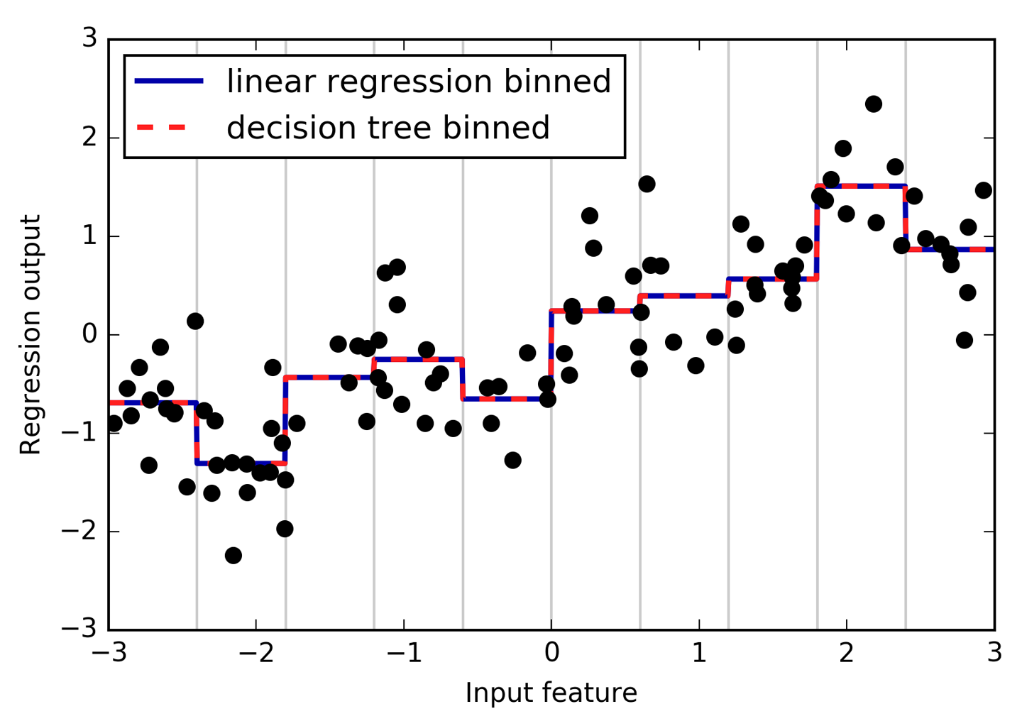
Figure 4-2. Comparing linear regression and decision tree regression on binned features
4.5 Interactions and Polynomials
Another way to enrich a feature representation, particularly for linear models, is adding interaction features and polynomial features of the original data. This kind of feature engineering is often used in statistical modeling, but it’s also common in many practical machine learning applications.
As a first example, look again at Figure 4-2. The linear model learned a constant value for
each bin in the wave dataset. We know, however, that linear models can learn
not only offsets, but also slopes. One way to add a slope to the
linear model on the binned data is to add the original feature (the x-axis in the plot) back in. This leads to an 11-dimensional dataset, as seen in Figure 4-3:
In[25]:
X_combined=np.hstack([X,X_binned])(X_combined.shape)
Out[25]:
(120, 11)
In[26]:
reg=LinearRegression().fit(X_combined,y)line_combined=np.hstack([line,line_binned])plt.plot(line,reg.predict(line_combined),label='linear regression combined')plt.vlines(kb.bin_edges_[0],-3,3,linewidth=1,alpha=.2)plt.legend(loc="best")plt.ylabel("Regression output")plt.xlabel("Input feature")plt.plot(X[:,0],y,'o',c='k')
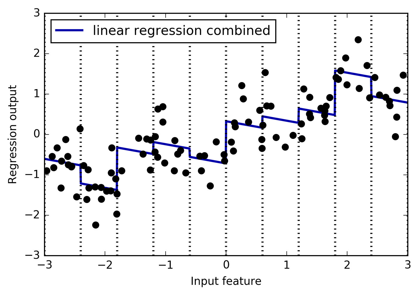
Figure 4-3. Linear regression using binned features and a single global slope
In this example, the model learned an offset for each bin, together with a slope. The learned slope is downward, and shared across all the bins—there is a single x-axis feature, which has a single slope. Because the slope is shared across all bins, it doesn’t seem to be very helpful. We would rather have a separate slope for each bin! We can achieve this by adding an interaction or product feature that indicates which bin a data point is in and where it lies on the x-axis. This feature is a product of the bin indicator and the original feature. Let’s create this dataset:
In[27]:
X_product=np.hstack([X_binned,X*X_binned])(X_product.shape)
Out[27]:
(120, 20)
The dataset now has 20 features: the indicators for which bin a data point is in, and a product of the original feature and the bin indicator. You can think of the product feature as a separate copy of the x-axis feature for each bin. It is the original feature within the bin, and zero everywhere else. Figure 4-4 shows the result of the linear model on this new representation:
In[28]:
reg=LinearRegression().fit(X_product,y)line_product=np.hstack([line_binned,line*line_binned])plt.plot(line,reg.predict(line_product),label='linear regression product')plt.vlines(kb.bin_edges_[0],-3,3,linewidth=1,alpha=.2)plt.plot(X[:,0],y,'o',c='k')plt.ylabel("Regression output")plt.xlabel("Input feature")plt.legend(loc="best")
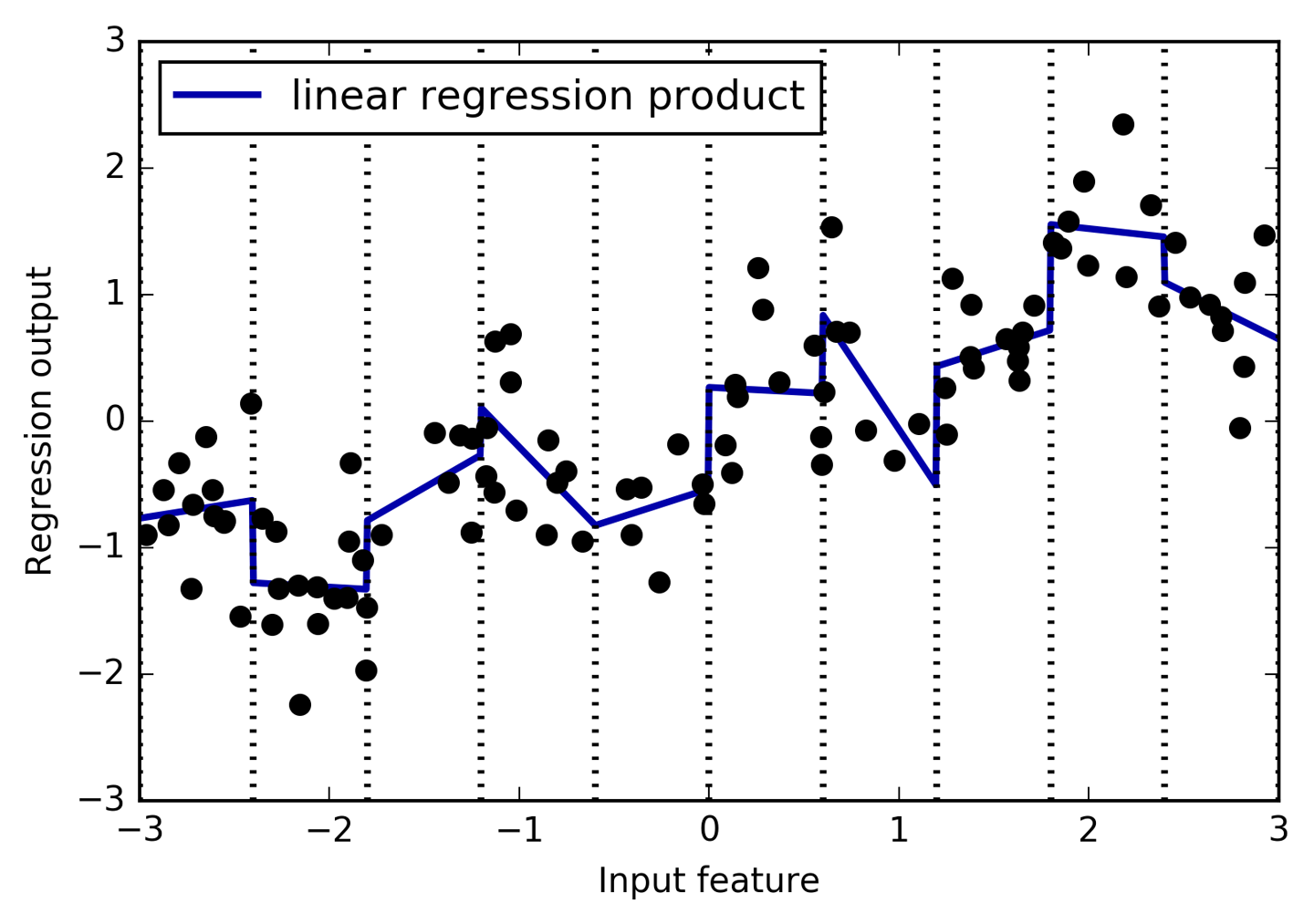
Figure 4-4. Linear regression with a separate slope per bin
As you can see, now each bin has its own offset and slope in this model.
Using binning is one way to expand a continuous feature. Another one is
to use polynomials of the original features. For a given feature x,
we might want to consider x ** 2, x ** 3, x ** 4, and so on. This
is implemented in PolynomialFeatures in the preprocessing module:
In[29]:
fromsklearn.preprocessingimportPolynomialFeatures# include polynomials up to x ** 10:# the default "include_bias=True" adds a feature that's constantly 1poly=PolynomialFeatures(degree=10,include_bias=False)poly.fit(X)X_poly=poly.transform(X)
Using a degree of 10 yields 10 features:
In[30]:
("X_poly.shape: {}".format(X_poly.shape))
Out[30]:
X_poly.shape: (120, 10)
Let’s compare the entries of X_poly to those of X:
In[31]:
("Entries of X:\n{}".format(X[:5]))("Entries of X_poly:\n{}".format(X_poly[:5]))
Out[31]:
Entries of X:
[[-0.753]
 [ 2.704]
 [ 1.392]
 [ 0.592]
 [-2.064]]
Entries of X_poly:
[[   -0.753     0.567    -0.427     0.321    -0.242     0.182    -0.137
      0.103    -0.078     0.058]
 [    2.704     7.313    19.777    53.482   144.632   391.125  1057.714
   2860.36   7735.232 20918.278]
 [    1.392     1.938     2.697     3.754     5.226     7.274    10.125
     14.094    19.618    27.307]
 [    0.592     0.35      0.207     0.123     0.073     0.043     0.025
      0.015     0.009     0.005]
 [   -2.064     4.26     -8.791    18.144   -37.448    77.289  -159.516
    329.222  -679.478  1402.367]]
You can obtain the semantics of the features by calling the
get_feature_names method, which provides the exponent for each
feature:
In[32]:
("Polynomial feature names:\n{}".format(poly.get_feature_names()))
Out[32]:
Polynomial feature names:
['x0', 'x0^2', 'x0^3', 'x0^4', 'x0^5', 'x0^6', 'x0^7', 'x0^8', 'x0^9', 'x0^10']
You can see that the first column of X_poly corresponds exactly to X,
while the other columns are the powers of the first entry. It’s
interesting to see how large some of the values can get. The second
row has entries above 20,000, orders of magnitude different from the
rest.
Using polynomial features together with a linear regression model yields the classical model of polynomial regression (see Figure 4-5):
In[33]:
reg=LinearRegression().fit(X_poly,y)line_poly=poly.transform(line)plt.plot(line,reg.predict(line_poly),label='polynomial linear regression')plt.plot(X[:,0],y,'o',c='k')plt.ylabel("Regression output")plt.xlabel("Input feature")plt.legend(loc="best")
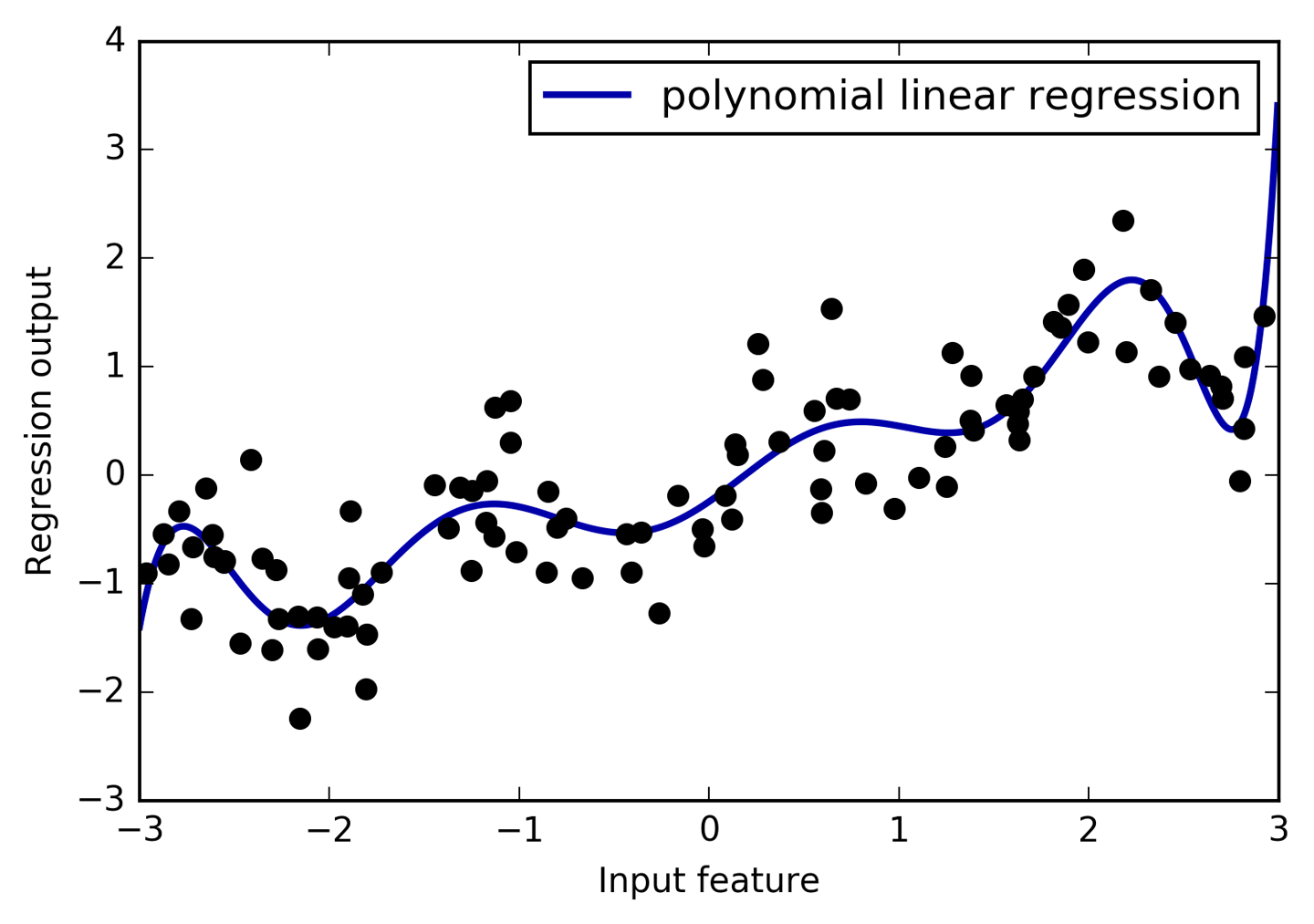
Figure 4-5. Linear regression with tenth-degree polynomial features
As you can see, polynomial features yield a very smooth fit on this one-dimensional data. However, polynomials of high degree tend to behave in extreme ways on the boundaries or in regions with little data.
As a comparison, here is a kernel SVM model learned on the original data, without any transformation (see Figure 4-6):
In[34]:
fromsklearn.svmimportSVRforgammain[1,10]:svr=SVR(gamma=gamma).fit(X,y)plt.plot(line,svr.predict(line),label='SVR gamma={}'.format(gamma))plt.plot(X[:,0],y,'o',c='k')plt.ylabel("Regression output")plt.xlabel("Input feature")plt.legend(loc="best")
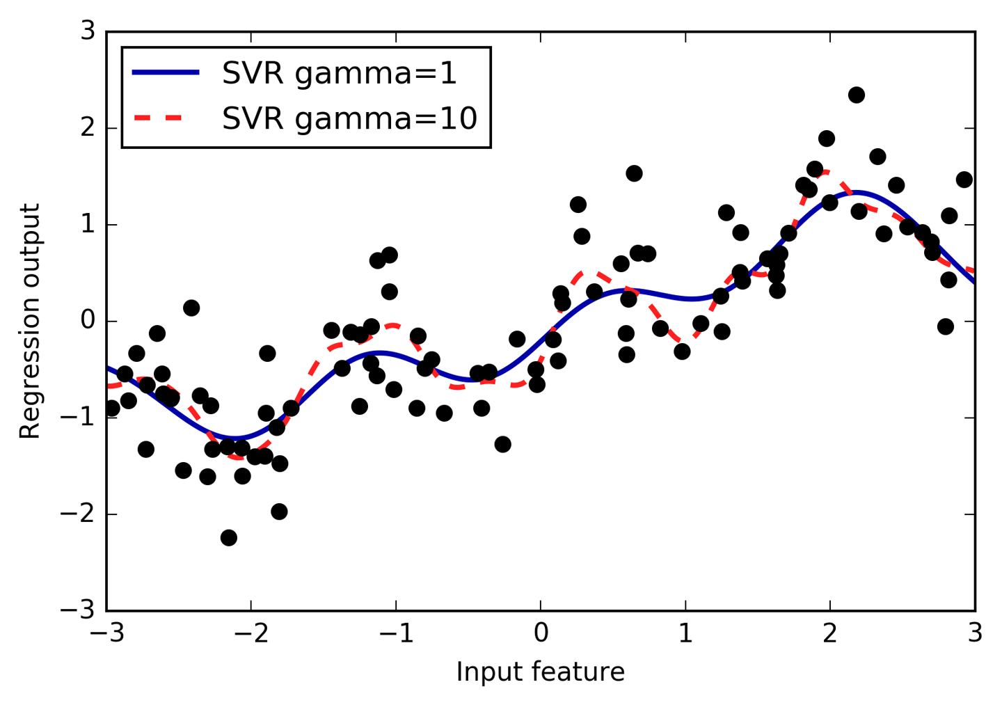
Figure 4-6. Comparison of different gamma parameters for an SVM with RBF kernel
Using a more complex model, a kernel SVM, we are able to learn a similarly complex prediction to the polynomial regression without an explicit transformation of the features.
As a more realistic application of interactions and polynomials, let’s
look again at the Boston Housing dataset. We already used polynomial
features on this dataset in Chapter 2. Now let’s have a look at how
these features were constructed, and at how much the polynomial features
help. First we load the data, and rescale it to be between 0 and 1 using
MinMaxScaler:
In[35]:
fromsklearn.datasetsimportload_bostonfromsklearn.model_selectionimporttrain_test_splitfromsklearn.preprocessingimportMinMaxScalerboston=load_boston()X_train,X_test,y_train,y_test=train_test_split(boston.data,boston.target,random_state=0)# rescale datascaler=MinMaxScaler()X_train_scaled=scaler.fit_transform(X_train)X_test_scaled=scaler.transform(X_test)
Now, we extract polynomial features and interactions up to a degree of 2:
In[36]:
poly=PolynomialFeatures(degree=2).fit(X_train_scaled)X_train_poly=poly.transform(X_train_scaled)X_test_poly=poly.transform(X_test_scaled)("X_train.shape: {}".format(X_train.shape))("X_train_poly.shape: {}".format(X_train_poly.shape))
Out[36]:
X_train.shape: (379, 13)
X_train_poly.shape: (379, 105)
The data originally had 13 features, which were expanded into 105
interaction features. These new features represent all possible
interactions between two different original features, as well as the
square of each original feature. degree=2 here means that we look at
all features that are the product of up to two original features. The
exact correspondence between input and output features can be found
using the get_feature_names method:
In[37]:
("Polynomial feature names:\n{}".format(poly.get_feature_names()))
Out[37]:
Polynomial feature names:
['1', 'x0', 'x1', 'x2', 'x3', 'x4', 'x5', 'x6', 'x7', 'x8', 'x9', 'x10',
'x11', 'x12', 'x0^2', 'x0 x1', 'x0 x2', 'x0 x3', 'x0 x4', 'x0 x5', 'x0 x6',
'x0 x7', 'x0 x8', 'x0 x9', 'x0 x10', 'x0 x11', 'x0 x12', 'x1^2', 'x1 x2',
'x1 x3', 'x1 x4', 'x1 x5', 'x1 x6', 'x1 x7', 'x1 x8', 'x1 x9', 'x1 x10',
'x1 x11', 'x1 x12', 'x2^2', 'x2 x3', 'x2 x4', 'x2 x5', 'x2 x6', 'x2 x7',
'x2 x8', 'x2 x9', 'x2 x10', 'x2 x11', 'x2 x12', 'x3^2', 'x3 x4', 'x3 x5',
'x3 x6', 'x3 x7', 'x3 x8', 'x3 x9', 'x3 x10', 'x3 x11', 'x3 x12', 'x4^2',
'x4 x5', 'x4 x6', 'x4 x7', 'x4 x8', 'x4 x9', 'x4 x10', 'x4 x11', 'x4 x12',
'x5^2', 'x5 x6', 'x5 x7', 'x5 x8', 'x5 x9', 'x5 x10', 'x5 x11', 'x5 x12',
'x6^2', 'x6 x7', 'x6 x8', 'x6 x9', 'x6 x10', 'x6 x11', 'x6 x12', 'x7^2',
'x7 x8', 'x7 x9', 'x7 x10', 'x7 x11', 'x7 x12', 'x8^2', 'x8 x9', 'x8 x10',
'x8 x11', 'x8 x12', 'x9^2', 'x9 x10', 'x9 x11', 'x9 x12', 'x10^2', 'x10 x11',
'x10 x12', 'x11^2', 'x11 x12', 'x12^2']
The first new feature is a constant feature, called "1" here. The next
13 features are the original features (called "x0" to "x12"). Then
follows the first feature squared ("x0^2") and combinations of the first
and the other features.
Let’s compare the performance using Ridge on the data with and without
interactions:
In[38]:
fromsklearn.linear_modelimportRidgeridge=Ridge().fit(X_train_scaled,y_train)("Score without interactions: {:.3f}".format(ridge.score(X_test_scaled,y_test)))ridge=Ridge().fit(X_train_poly,y_train)("Score with interactions: {:.3f}".format(ridge.score(X_test_poly,y_test)))
Out[38]:
Score without interactions: 0.621
Score with interactions: 0.753
Clearly, the interactions and polynomial features gave us a good boost in
performance when using Ridge. When using a more complex model like a
random forest, the story is a bit different, though:
In[39]:
fromsklearn.ensembleimportRandomForestRegressorrf=RandomForestRegressor(n_estimators=100).fit(X_train_scaled,y_train)("Score without interactions: {:.3f}".format(rf.score(X_test_scaled,y_test)))rf=RandomForestRegressor(n_estimators=100).fit(X_train_poly,y_train)("Score with interactions: {:.3f}".format(rf.score(X_test_poly,y_test)))
Out[39]:
Score without interactions: 0.798
Score with interactions: 0.765
You can see that even without additional features, the random forest
beats the performance of Ridge. Adding interactions and polynomials
actually decreases performance slightly.
4.6 Univariate Nonlinear Transformations
We just saw that adding squared or cubed features can help linear models
for regression. There are other transformations that often prove useful
for transforming certain features: in particular, applying mathematical
functions like log, exp, or sin. While tree-based models only care
about the ordering of the features, linear models and neural networks
are very tied to the scale and distribution of each feature, and if
there is a nonlinear relation between the feature and the target, that
becomes hard to model—particularly in regression. The functions log
and exp can help by adjusting the relative scales in the data so that
they can be captured better by a linear model or neural network. We saw
an application of that in Chapter 2 with the memory price data. The
sin and cos functions can come in handy when dealing with data that
encodes periodic patterns.
Most models work best when each feature (and in regression also the
target) is loosely Gaussian distributed—that is, a histogram of each
feature should have something resembling the familiar “bell curve” shape.
Using transformations like log and exp is a hacky but simple and
efficient way to achieve this. A particularly common case when such a
transformation can be helpful is when dealing with integer count data.
By count data, we mean features like “how often did user A log in?”
Counts are never negative, and often follow particular statistical
patterns. We are using a synthetic dataset of counts here that has
properties similar to those you can find in the wild. The features are
all integer-valued, while the response is continuous:
In[40]:
rnd=np.random.RandomState(0)X_org=rnd.normal(size=(1000,3))w=rnd.normal(size=3)X=rnd.poisson(10*np.exp(X_org))y=np.dot(X_org,w)
Let’s look at the first 10 entries of the first feature. All are integer values and positive, but apart from that it’s hard to make out a particular pattern.
If we count the appearance of each value, the distribution of values becomes clearer:
In[41]:
("Number of feature appearances:\n{}".format(np.bincount(X[:,0])))
Out[41]:
Number of feature appearances:
[28 38 68 48 61 59 45 56 37 40 35 34 36 26 23 26 27 21 23 23 18 21 10  9 17
  9  7 14 12  7  3  8  4  5  5  3  4  2  4  1  1  3  2  5  3  8  2  5  2  1
  2  3  3  2  2  3  3  0  1  2  1  0  0  3  1  0  0  0  1  3  0  1  0  2  0
  1  1  0  0  0  0  1  0  0  2  2  0  1  1  0  0  0  0  1  1  0  0  0  0  0
  0  0  1  0  0  0  0  0  1  1  0  0  1  0  0  0  0  0  0  0  1  0  0  0  0
  1  0  0  0  0  0  0  0  0  0  0  0  0  0  0  1]
The value 2 seems to be the most common, with 68 appearances (bincount
always starts at 0), and the counts for higher values fall quickly.
However, there are some very high values, like 84 and 85, that are appearing twice. We
visualize the counts in Figure 4-7:
In[42]:
bins=np.bincount(X[:,0])plt.bar(range(len(bins)),bins,color='grey')plt.ylabel("Number of appearances")plt.xlabel("Value")
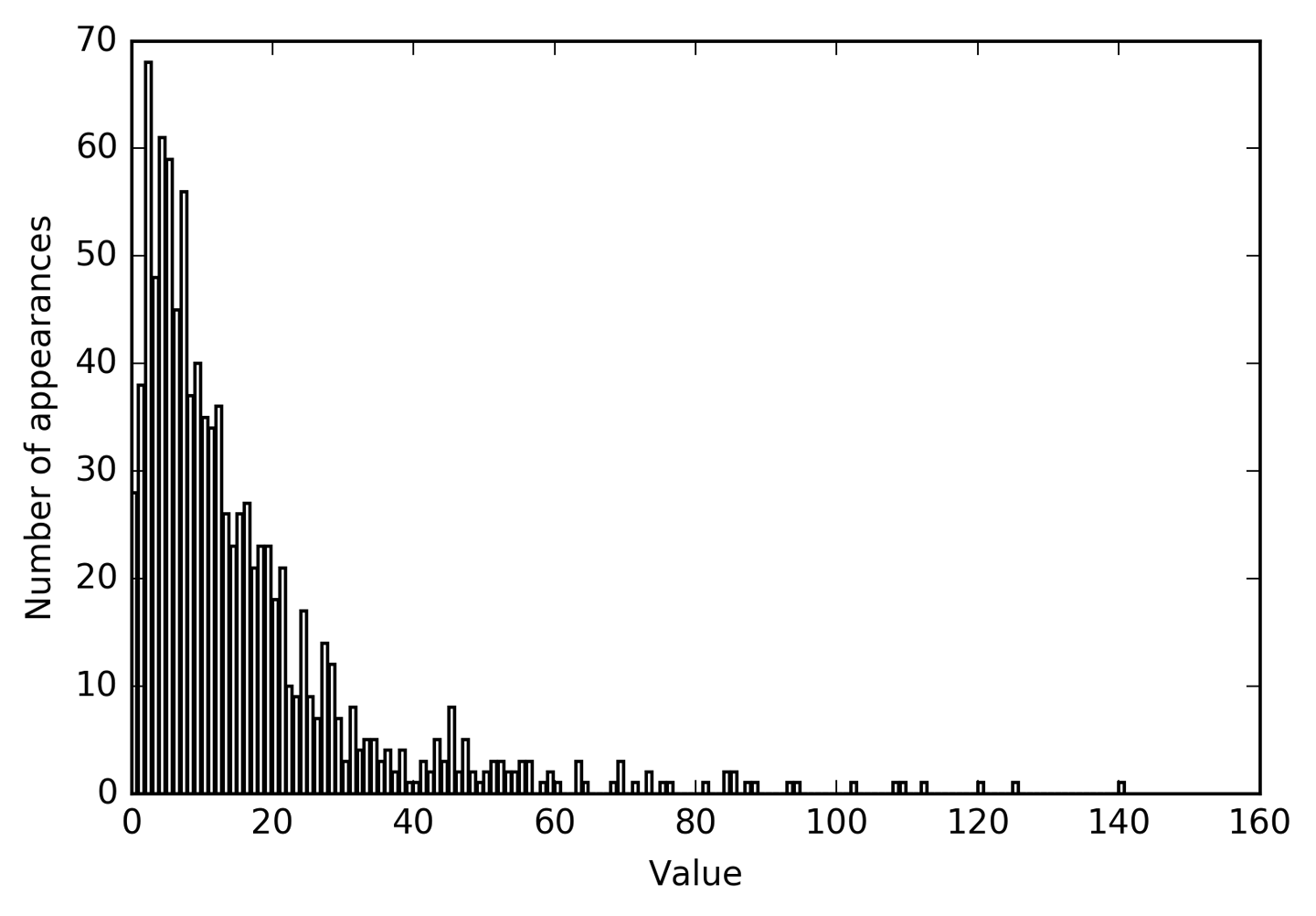
Figure 4-7. Histogram of feature values for X[0]
Features X[:, 1] and X[:, 2] have similar properties. This kind of
distribution of values (many small ones and a few very large ones) is
very common in practice.2 However, it is something most
linear models can’t handle very well. Let’s try to fit a ridge
regression to this model:
In[43]:
fromsklearn.linear_modelimportRidgeX_train,X_test,y_train,y_test=train_test_split(X,y,random_state=0)score=Ridge().fit(X_train,y_train).score(X_test,y_test)("Test score: {:.3f}".format(score))
Out[43]:
Test score: 0.622
As you can see from the relatively low R2 score, Ridge was not able to really capture the relationship between X and y. Applying a logarithmic transformation can help, though. Because the
value 0 appears in the data (and the logarithm is not defined at 0), we
can’t actually just apply log, but we have to compute log(X + 1):
In[44]:
X_train_log=np.log(X_train+1)X_test_log=np.log(X_test+1)
After the transformation, the distribution of the data is less asymmetrical and doesn’t have very large outliers anymore (see Figure 4-8):
In[45]:
plt.hist(X_train_log[:,0],bins=25,color='gray')plt.ylabel("Number of appearances")plt.xlabel("Value")
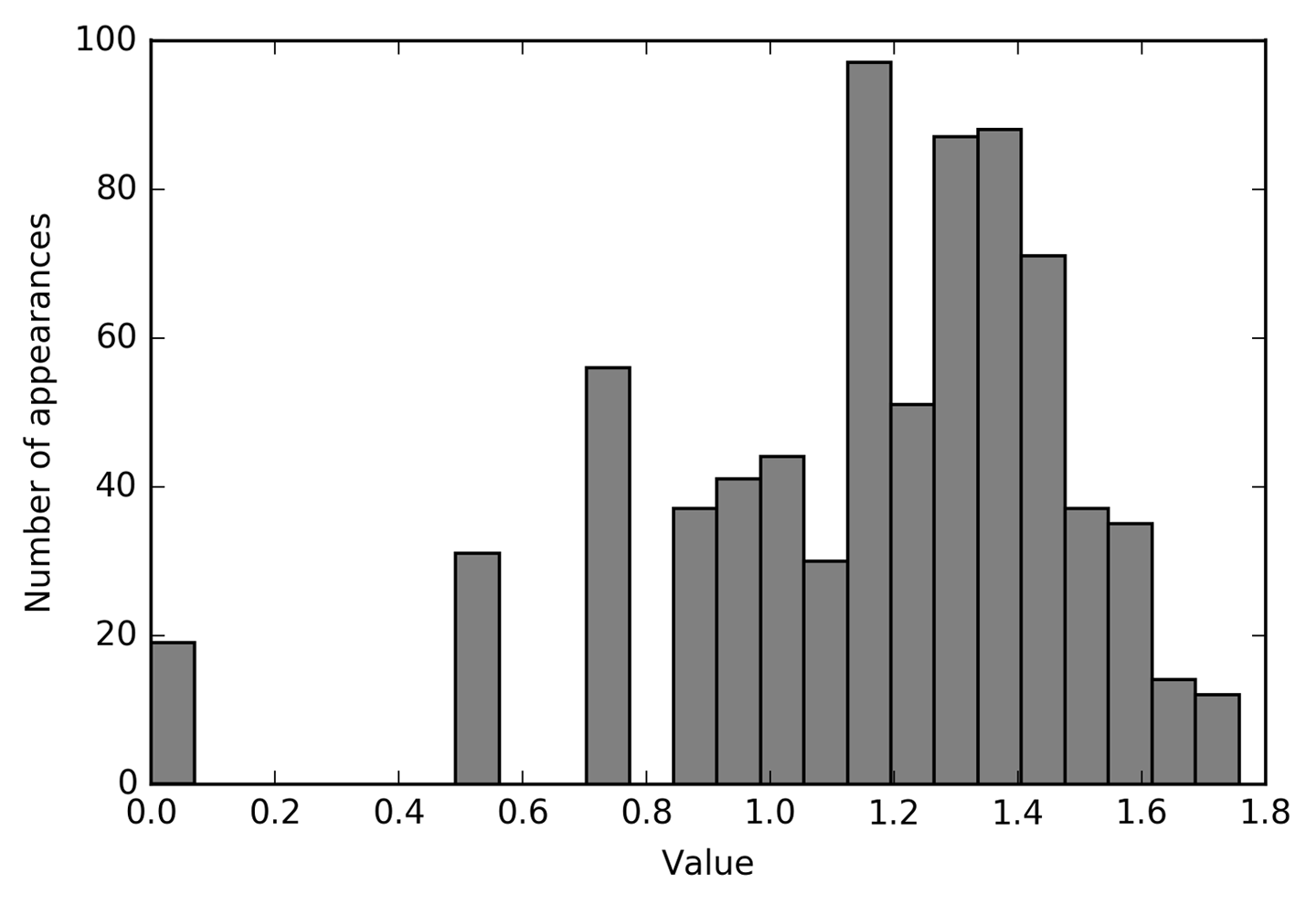
Figure 4-8. Histogram of feature values for X[0] after logarithmic transformation
Building a ridge model on the new data provides a much better fit:
In[46]:
score=Ridge().fit(X_train_log,y_train).score(X_test_log,y_test)("Test score: {:.3f}".format(score))
Out[46]:
Test score: 0.875
Finding the transformation that works best for each combination of
dataset and model is somewhat of an art. In this example, all the
features had the same properties. This is rarely the case in practice,
and usually only a subset of the features should be transformed, or
sometimes each feature needs to be transformed in a different way. As we
mentioned earlier, these kinds of transformations are irrelevant for
tree-based models but might be essential for linear models. Sometimes
it is also a good idea to transform the target variable y in
regression. Trying to predict counts (say, number of orders) is a fairly
common task, and using the log(y + 1) transformation often helps.3
As you saw in the previous examples, binning, polynomials, and interactions can have a huge influence on how models perform on a given dataset. This is particularly true for less complex models like linear models and naive Bayes models. Tree-based models, on the other hand, are often able to discover important interactions themselves, and don’t require transforming the data explicitly most of the time. Other models, like SVMs, nearest neighbors, and neural networks, might sometimes benefit from using binning, interactions, or polynomials, but the implications there are usually much less clear than in the case of linear models.
4.7 Automatic Feature Selection
With so many ways to create new features, you might get tempted to increase the dimensionality of the data way beyond the number of original features. However, adding more features makes all models more complex, and so increases the chance of overfitting. When adding new features, or with high-dimensional datasets in general, it can be a good idea to reduce the number of features to only the most useful ones, and discard the rest. This can lead to simpler models that generalize better. But how can you know how good each feature is? There are three basic strategies: univariate statistics, model-based selection, and iterative selection. We will discuss all three of them in detail. All of these methods are supervised methods, meaning they need the target for fitting the model. This means we need to split the data into training and test sets, and fit the feature selection only on the training part of the data.
4.7.1 Univariate Statistics
In univariate statistics, we compute whether there is a statistically significant relationship between each feature and the target. Then the features that are related with the highest confidence are selected. In the case of classification, this is also known as analysis of variance (ANOVA). A key property of these tests is that they are univariate, meaning that they only consider each feature individually. Consequently, a feature will be discarded if it is only informative when combined with another feature. Univariate tests are often very fast to compute, and don’t require building a model. On the other hand, they are completely independent of the model that you might want to apply after the feature selection.
To use univariate feature selection in scikit-learn, you need to choose
a test, usually either f_classif (the default) for classification or
f_regression for regression, and a method to discard features based on
the p-values determined in the test. All methods for discarding
parameters use a threshold to discard all features with too high a
p-value (which means they are unlikely to be related to the target).
The methods differ in how they compute this threshold, with the simplest
ones being SelectKBest, which selects a fixed number k of features,
and SelectPercentile, which selects a fixed percentage of features.
Let’s apply the feature selection for classification on the cancer
dataset. To make the task a bit harder, we’ll add some noninformative
noise features to the data. We expect the feature selection to be able
to identify the features that are noninformative and remove them:
In[47]:
fromsklearn.datasetsimportload_breast_cancerfromsklearn.feature_selectionimportSelectPercentilefromsklearn.model_selectionimporttrain_test_splitcancer=load_breast_cancer()# get deterministic random numbersrng=np.random.RandomState(42)noise=rng.normal(size=(len(cancer.data),50))# add noise features to the data# the first 30 features are from the dataset, the next 50 are noiseX_w_noise=np.hstack([cancer.data,noise])X_train,X_test,y_train,y_test=train_test_split(X_w_noise,cancer.target,random_state=0,test_size=.5)# use f_classif (the default) and SelectPercentile to select 50% of featuresselect=SelectPercentile(percentile=50)select.fit(X_train,y_train)# transform training setX_train_selected=select.transform(X_train)("X_train.shape: {}".format(X_train.shape))("X_train_selected.shape: {}".format(X_train_selected.shape))
Out[47]:
X_train.shape: (284, 80)
X_train_selected.shape: (284, 40)
As you can see, the number of features was reduced from 80 to 40 (50
percent of the original number of features). We can find out which
features have been selected using the get_support method, which
returns a Boolean mask of the selected features (visualized in Figure 4-9):
In[48]:
mask=select.get_support()(mask)# visualize the mask -- black is True, white is Falseplt.matshow(mask.reshape(1,-1),cmap='gray_r')plt.xlabel("Sample index")plt.yticks(())
Out[48]:
[ True  True  True  True  True  True  True  True  True False  True False
  True  True  True  True  True  True False False  True  True  True  True
  True  True  True  True  True  True False False False  True False  True
 False False  True False False False False  True False False  True False
 False  True False  True False False False False False False  True False
  True False False False False  True False  True False False False False
  True  True False  True False False False False]

Figure 4-9. Features selected by SelectPercentile
As you can see from the visualization of the mask, most of the selected features are the original features, and most of the noise features were removed. However, the recovery of the original features is not perfect. Let’s compare the performance of logistic regression on all features against the performance using only the selected features:
In[49]:
fromsklearn.linear_modelimportLogisticRegression# transform test dataX_test_selected=select.transform(X_test)lr=LogisticRegression()lr.fit(X_train,y_train)("Score with all features: {:.3f}".format(lr.score(X_test,y_test)))lr.fit(X_train_selected,y_train)("Score with only selected features: {:.3f}".format(lr.score(X_test_selected,y_test)))
Out[49]:
Score with all features: 0.930
Score with only selected features: 0.940
In this case, removing the noise features improved performance, even though some of the original features were lost. This was a very simple synthetic example, and outcomes on real data are usually mixed. Univariate feature selection can still be very helpful, though, if there is such a large number of features that building a model on them is infeasible, or if you suspect that many features are completely uninformative.
4.7.2 Model-Based Feature Selection
Model-based feature selection uses a supervised machine learning model
to judge the importance of each feature, and keeps only the most
important ones. The supervised model that is used for feature selection
doesn’t need to be the same model that is used for the final supervised
modeling. The feature selection model needs to provide
some measure of importance for each feature, so that they can be ranked
by this measure. Decision trees and decision tree–based models provide a feature_importances_ attribute, which directly encodes the importance of each feature. Linear models have coefficients, which can also be used to capture feature importances by considering the absolute values. As we saw in
Chapter 2, linear models with L1 penalty learn sparse coefficients,
which only use a small subset of features. This can be viewed as a form
of feature selection for the model itself, but can also be used as a
preprocessing step to select features for another model. In contrast to
univariate selection, model-based selection considers all features at
once, and so can capture interactions (if the model can capture them).
To use model-based feature selection, we need to use the
SelectFromModel transformer:
In[50]:
fromsklearn.feature_selectionimportSelectFromModelfromsklearn.ensembleimportRandomForestClassifierselect=SelectFromModel(RandomForestClassifier(n_estimators=100,random_state=42),threshold="median")
The SelectFromModel class selects all features that have an importance
measure of the feature (as provided by the supervised model) greater
than the provided threshold. To get a comparable result to what we got
with univariate feature selection, we used the median as a threshold, so
that half of the features will be selected. We use a random forest
classifier with 100 trees to compute the feature importances. This is a
quite complex model and much more powerful than using univariate tests.
Now let’s actually fit the model:
In[51]:
select.fit(X_train,y_train)X_train_l1=select.transform(X_train)("X_train.shape: {}".format(X_train.shape))("X_train_l1.shape: {}".format(X_train_l1.shape))
Out[51]:
X_train.shape: (284, 80)
X_train_l1.shape: (284, 40)
Again, we can have a look at the features that were selected (Figure 4-10):
In[52]:
mask=select.get_support()# visualize the mask -- black is True, white is Falseplt.matshow(mask.reshape(1,-1),cmap='gray_r')plt.xlabel("Sample index")plt.yticks(())

Figure 4-10. Features selected by SelectFromModel using the RandomForestClassifier
This time, all but two of the original features were selected. Because we specified to select 40 features, some of the noise features are also selected. Let’s take a look at the performance:
In[53]:
X_test_l1=select.transform(X_test)score=LogisticRegression().fit(X_train_l1,y_train).score(X_test_l1,y_test)("Test score: {:.3f}".format(score))
Out[53]:
Test score: 0.951
With the better feature selection, we also gained some improvements here.
4.7.3 Iterative Feature Selection
In univariate testing we used no model, while in model-based selection we used a single model to select features. In iterative feature selection, a series of models are built, with varying numbers of features. There are two basic methods: starting with no features and adding features one by one until some stopping criterion is reached, or starting with all features and removing features one by one until some stopping criterion is reached. Because a series of models are built, these methods are much more computationally expensive than the methods we discussed previously. One particular method of this kind is recursive feature elimination (RFE), which starts with all features, builds a model, and discards the least important feature according to the model. Then a new model is built using all but the discarded feature, and so on until only a prespecified number of features are left. For this to work, the model used for selection needs to provide some way to determine feature importance, as was the case for the model-based selection. Here, we use the same random forest model that we used earlier, and get the results shown in Figure 4-11:
In[54]:
fromsklearn.feature_selectionimportRFEselect=RFE(RandomForestClassifier(n_estimators=100,random_state=42),n_features_to_select=40)select.fit(X_train,y_train)# visualize the selected features:mask=select.get_support()plt.matshow(mask.reshape(1,-1),cmap='gray_r')plt.xlabel("Sample index")plt.yticks(())

Figure 4-11. Features selected by recursive feature elimination with the random forest classifier model
The feature selection got better compared to the univariate and model-based selection, but one feature was still missed. Running this code also takes significantly longer than that for the model-based selection, because a random forest model is trained 40 times, once for each feature that is dropped. Let’s test the accuracy of the logistic regression model when using RFE for feature selection:
In[55]:
X_train_rfe=select.transform(X_train)X_test_rfe=select.transform(X_test)score=LogisticRegression().fit(X_train_rfe,y_train).score(X_test_rfe,y_test)("Test score: {:.3f}".format(score))
Out[55]:
Test score: 0.951
We can also use the model used inside the RFE to make predictions. This uses only the feature set that was selected:
In[56]:
("Test score: {:.3f}".format(select.score(X_test,y_test)))
Out[56]:
Test score: 0.951
Here, the performance of the random forest used inside the RFE is the same as that achieved by training a logistic regression model on top of the selected features. In other words, once we’ve selected the right features, the linear model performs as well as the random forest.
If you are unsure when selecting what to use as input to your machine learning algorithms, automatic feature selection can be quite helpful. It is also great for reducing the amount of features needed—for example, to speed up prediction or to allow for more interpretable models. In most real-world cases, applying feature selection is unlikely to provide large gains in performance. However, it is still a valuable tool in the toolbox of the feature engineer.
4.8 Utilizing Expert Knowledge
Feature engineering is often an important place to use expert knowledge for a particular application. While the purpose of machine learning in many cases is to avoid having to create a set of expert-designed rules, that doesn’t mean that prior knowledge of the application or domain should be discarded. Often, domain experts can help in identifying useful features that are much more informative than the initial representation of the data. Imagine you work for a travel agency and want to predict flight prices. Let’s say you have a record of prices together with dates, airlines, start locations, and destinations. A machine learning model might be able to build a decent model from that. Some important factors in flight prices, however, cannot be learned. For example, flights are usually more expensive during peak vacation months and around holidays. While the dates of some holidays (like Christmas) are fixed, and their effect can therefore be learned from the date, others might depend on the phases of the moon (like Hanukkah and Easter) or be set by authorities (like school holidays). These events cannot be learned from the data if each flight is only recorded using the (Gregorian) date. However, it is easy to add a feature that encodes whether a flight was on, preceding, or following a public or school holiday. In this way, prior knowledge about the nature of the task can be encoded in the features to aid a machine learning algorithm. Adding a feature does not force a machine learning algorithm to use it, and even if the holiday information turns out to be noninformative for flight prices, augmenting the data with this information doesn’t hurt.
We’ll now look at one particular case of using expert knowledge—though in this case it might be more rightfully called “common sense.” The task is predicting bicycle rentals in front of Andreas’s house.
In New York, Citi Bike operates a network of bicycle rental stations with a subscription system. The stations are all over the city and provide a convenient way to get around. Bike rental data is made public in an anonymized form and has been analyzed in various ways. The task we want to solve is to predict for a given time and day how many people will rent a bike in front of Andreas’s house—so he knows if any bikes will be left for him.
We first load the data for August 2015 for this particular station as a
pandas DataFrame. We resample the data into three-hour intervals to obtain
the main trends for each day:
In[57]:
citibike=mglearn.datasets.load_citibike()
In[58]:
("Citi Bike data:\n{}".format(citibike.head()))
Out[58]:
Citi Bike data:
starttime
2015-08-01 00:00:00     3
2015-08-01 03:00:00     0
2015-08-01 06:00:00     9
2015-08-01 09:00:00    41
2015-08-01 12:00:00    39
Freq: 3H, Name: one, dtype: int64
The following example shows a visualization of the rental frequencies for the whole month (Figure 4-12):
In[59]:
plt.figure(figsize=(10,3))xticks=pd.date_range(start=citibike.index.min(),end=citibike.index.max(),freq='D')plt.xticks(xticks.astype("int"),xticks.strftime("%a%m-%d"),rotation=90,ha="left")plt.plot(citibike,linewidth=1)plt.xlabel("Date")plt.ylabel("Rentals")
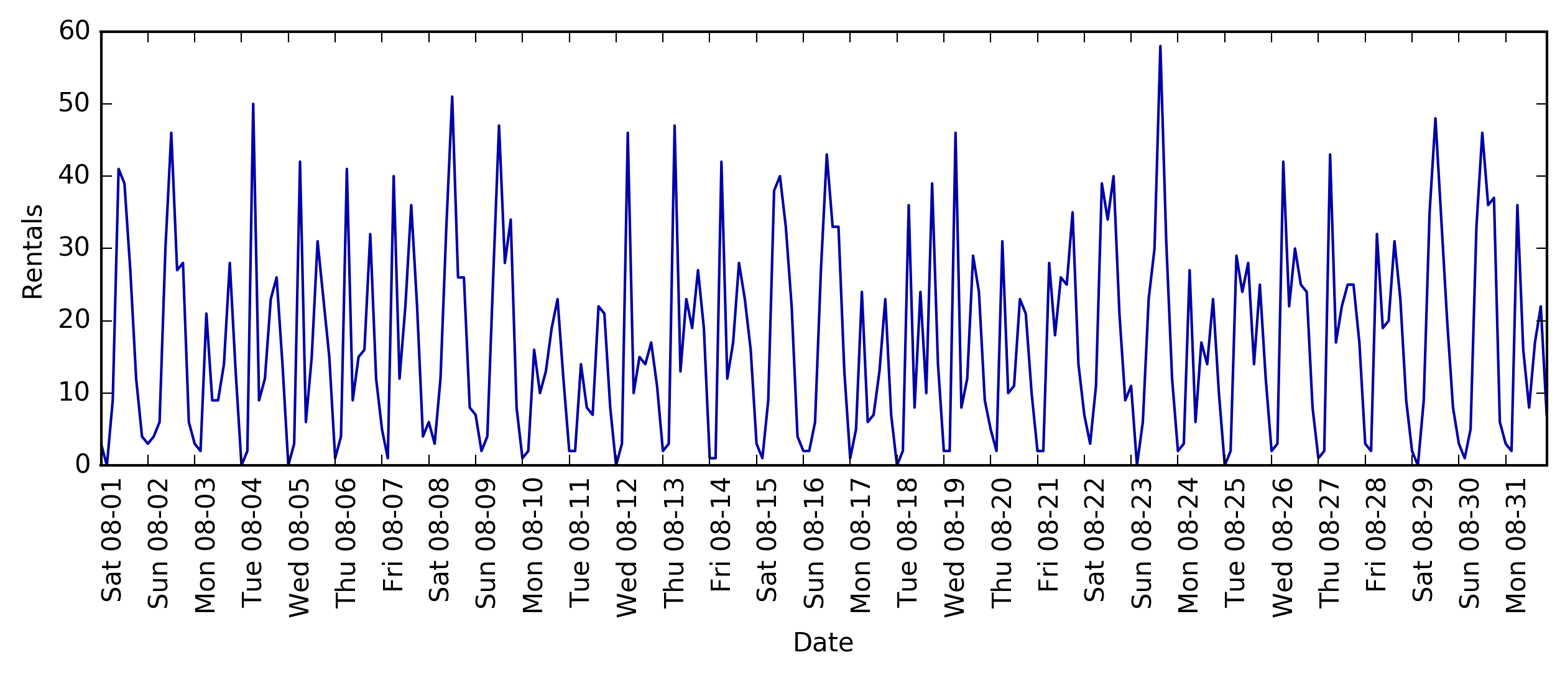
Figure 4-12. Number of bike rentals over time for a selected Citi Bike station
Looking at the data, we can clearly distinguish day and night for each 24-hour interval. The patterns for weekdays and weekends also seem to be quite different. When evaluating a prediction task on a time series like this, we usually want to learn from the past and predict for the future. This means when doing a split into a training and a test set, we want to use all the data up to a certain date as the training set and all the data past that date as the test set. This is how we would usually use time series prediction: given everything that we know about rentals in the past, what do we think will happen tomorrow? We will use the first 184 data points, corresponding to the first 23 days, as our training set, and the remaining 64 data points, corresponding to the remaining 8 days, as our test set.
The only feature that we are using in our prediction task is the date
and time when a particular number of rentals occurred. So, the input
feature is the date and time—say, 2015-08-01 00:00:00—and the output is the
number of rentals in the following three hours (three in this case, according to our DataFrame).
A (surprisingly) common way that dates are stored on computers is using POSIX time, which is the number of seconds since January 1970 00:00:00 (aka the beginning of Unix time). As a first try, we can use this single integer feature as our data representation:
In[60]:
# extract the target values (number of rentals)y=citibike.values# convert to POSIX time by dividing by 10**9X=citibike.index.astype("int64").values.reshape(-1,1)//10**9
We first define a function to split the data into training and test sets, build the model, and visualize the result:
In[61]:
# use the first 184 data points for training, and the rest for testingn_train=184# function to evaluate and plot a regressor on a given feature setdefeval_on_features(features,target,regressor):# split the given features into a training and a test setX_train,X_test=features[:n_train],features[n_train:]# also split the target arrayy_train,y_test=target[:n_train],target[n_train:]regressor.fit(X_train,y_train)("Test-set R^2: {:.2f}".format(regressor.score(X_test,y_test)))y_pred=regressor.predict(X_test)y_pred_train=regressor.predict(X_train)plt.figure(figsize=(10,3))plt.xticks(range(0,len(X),8),xticks.strftime("%a%m-%d"),rotation=90,ha="left")plt.plot(range(n_train),y_train,label="train")plt.plot(range(n_train,len(y_test)+n_train),y_test,'-',label="test")plt.plot(range(n_train),y_pred_train,'--',label="prediction train")plt.plot(range(n_train,len(y_test)+n_train),y_pred,'--',label="prediction test")plt.legend(loc=(1.01,0))plt.xlabel("Date")plt.ylabel("Rentals")
We saw earlier that random forests require very little preprocessing of the
data, which makes this seem like a good model to start with. We use the
POSIX time feature X and pass a random forest regressor to our
eval_on_features function. Figure 4-13 shows the result:
In[62]:
fromsklearn.ensembleimportRandomForestRegressorregressor=RandomForestRegressor(n_estimators=100,random_state=0)eval_on_features(X,y,regressor)
Out[62]:
Test-set R^2: -0.04
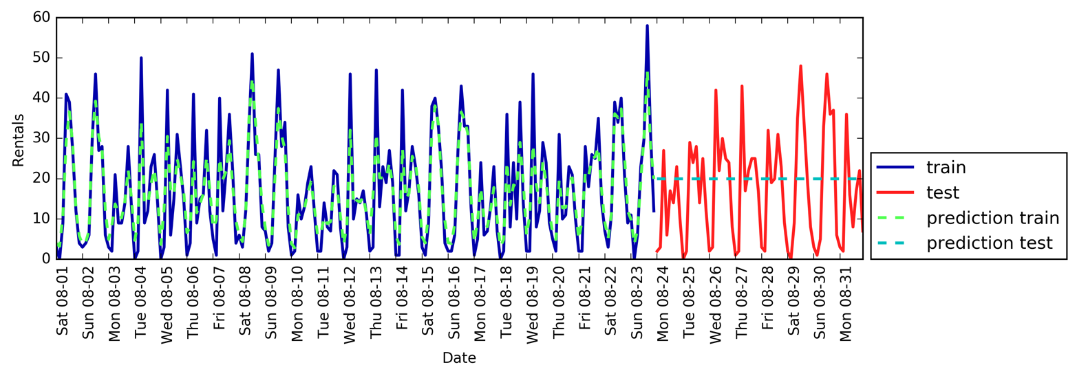
Figure 4-13. Predictions made by a random forest using only the POSIX time
The predictions on the training set are quite good, as is usual for random forests. However, for the test set, a constant line is predicted. The R2 is –0.04, which means that we learned nothing. What happened?
The problem lies in the combination of our feature and the random forest. The value of the POSIX time feature for the test set is outside of the range of the feature values in the training set: the points in the test set have timestamps that are later than all the points in the training set. Trees, and therefore random forests, cannot extrapolate to feature ranges outside the training set. The result is that the model simply predicts the target value of the closest point in the training set—which is the last time it observed any data.
Clearly we can do better than this. This is where our “expert knowledge” comes in. From looking at the rental figures in the training data, two factors seem to be very important: the time of day and the day of the week. So, let’s add these two features. We can’t really learn anything from the POSIX time, so we drop that feature. First, let’s use only the hour of the day. As Figure 4-14 shows, now the predictions have the same pattern for each day of the week:
In[63]:
X_hour=citibike.index.hour.values.reshape(-1,1)eval_on_features(X_hour,y,regressor)
Out[63]:
Test-set R^2: 0.60
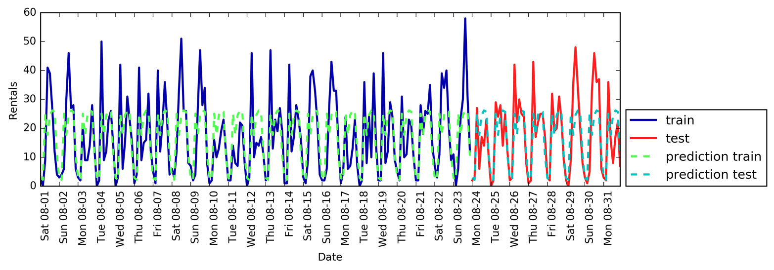
Figure 4-14. Predictions made by a random forest using only the hour of the day
The R2 is already much better, but the predictions clearly miss the weekly pattern. Now let’s also add the day of the week (see Figure 4-15):
In[64]:
X_hour_week=np.hstack([citibike.index.dayofweek.values.reshape(-1,1),citibike.index.hour.values.reshape(-1,1)])eval_on_features(X_hour_week,y,regressor)
Out[64]:
Test-set R^2: 0.84
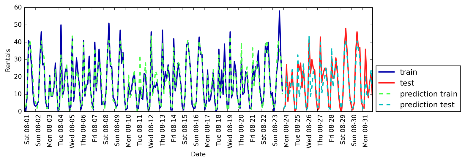
Figure 4-15. Predictions with a random forest using day of week and hour of day features
Now we have a model that captures the periodic behavior by considering the day of week and time of day. It has an R2 of 0.84, and shows
pretty good predictive performance. What this model likely is learning
is the mean number of rentals for each combination of weekday and time
of day from the first 23 days of August. This actually does not require
a complex model like a random forest, so let’s try with a simpler model, LinearRegression (see Figure 4-16):
In[65]:
fromsklearn.linear_modelimportLinearRegressioneval_on_features(X_hour_week,y,LinearRegression())
Out[65]:
Test-set R^2: 0.13
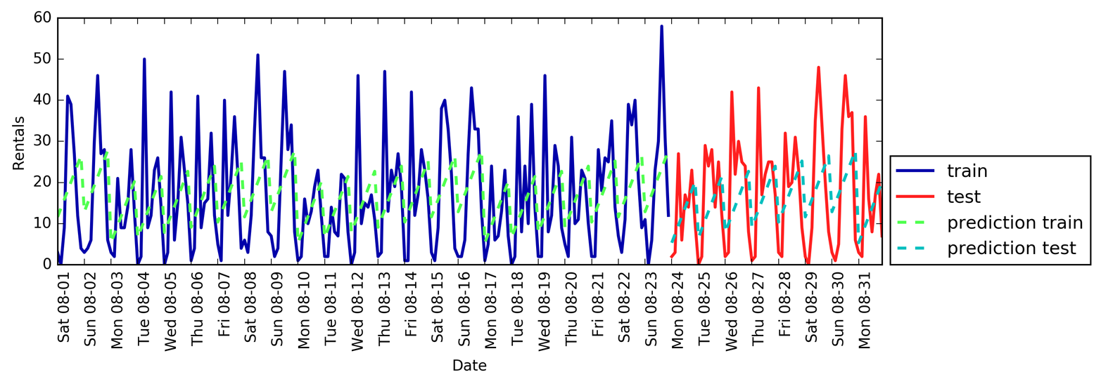
Figure 4-16. Predictions made by linear regression using day of week and hour of day as features
LinearRegression
works much worse, and the periodic pattern looks odd.
The reason for this is that we encoded day of week and time of
day using integers, which are interpreted as continuous variables.
Therefore, the linear model can only learn a linear function of the time
of day—and it learned that later in the day, there are more rentals.
However, the patterns are much more complex than that. We can capture this
by interpreting the integers as categorical variables, by transforming
them using OneHotEncoder (see Figure 4-17):
In[66]:
enc=OneHotEncoder()X_hour_week_onehot=enc.fit_transform(X_hour_week).toarray()
In[67]:
eval_on_features(X_hour_week_onehot,y,Ridge())
Out[67]:
Test-set R^2: 0.62
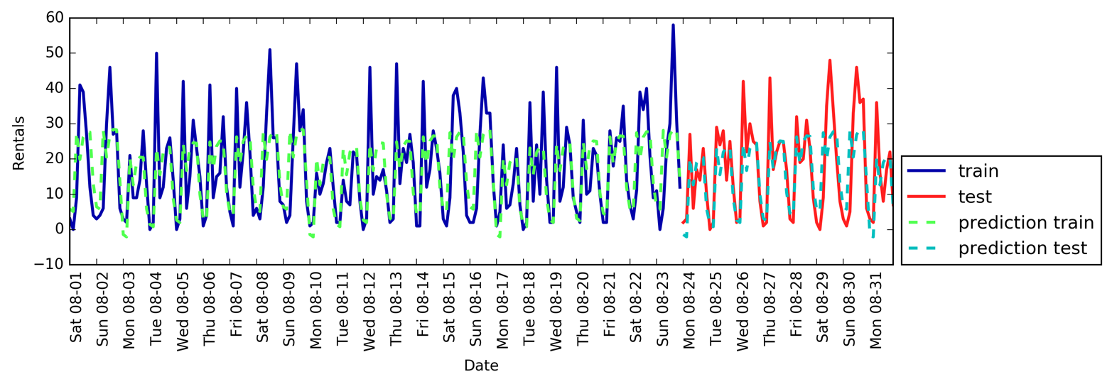
Figure 4-17. Predictions made by linear regression using a one-hot encoding of hour of day and day of week
This gives us a much better match than the continuous feature encoding. Now the linear model learns one coefficient for each day of the week, and one coefficient for each time of the day. That means that the “time of day” pattern is shared over all days of the week, though.
Using interaction features, we can allow the model to learn one coefficient for each combination of day and time of day (see Figure 4-18):
In[68]:
poly_transformer=PolynomialFeatures(degree=2,interaction_only=True,include_bias=False)X_hour_week_onehot_poly=poly_transformer.fit_transform(X_hour_week_onehot)lr=Ridge()eval_on_features(X_hour_week_onehot_poly,y,lr)
Out[68]:
Test-set R^2: 0.85
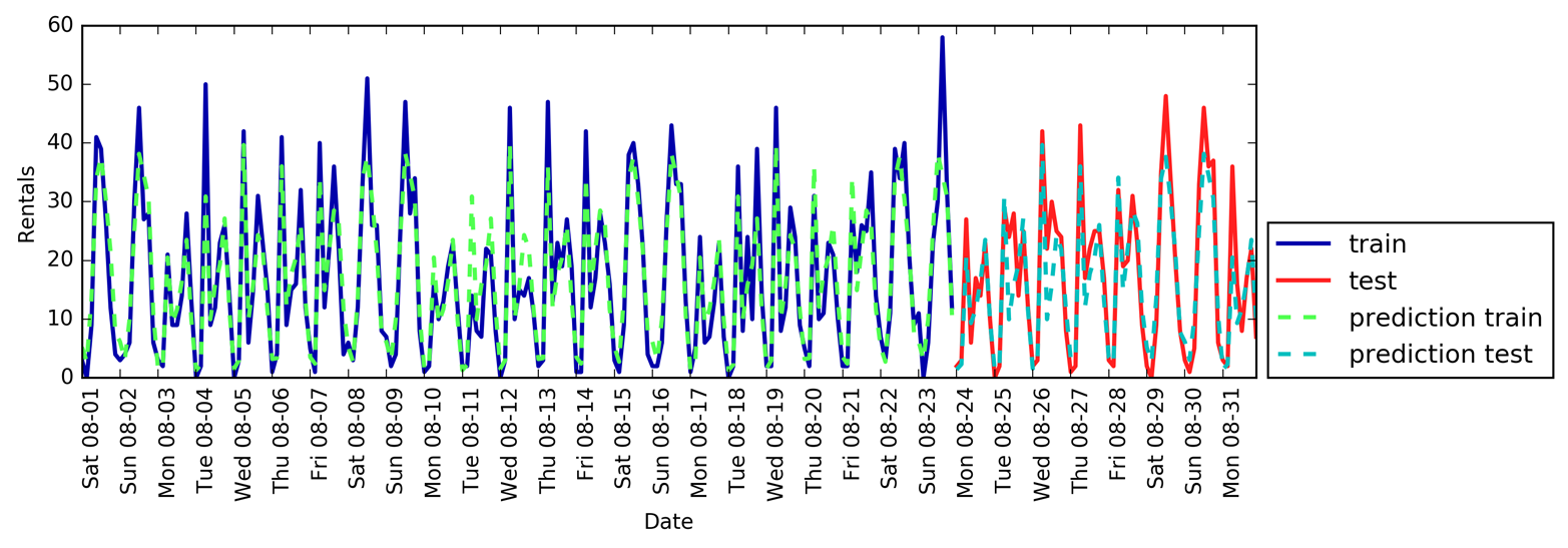
Figure 4-18. Predictions made by linear regression using a product of the day of week and hour of day features
This transformation finally yields a model that performs similarly well to the random forest. A big benefit of this model is that it is very clear what is learned: one coefficient for each day and time. We can simply plot the coefficients learned by the model, something that would not be possible for the random forest.
First, we create feature names for the hour and day features:
In[69]:
hour=["%02d:00"%iforiinrange(0,24,3)]day=["Mon","Tue","Wed","Thu","Fri","Sat","Sun"]features=day+hour
Then we name all the interaction features extracted by
PolynomialFeatures, using the get_feature_names method, and keep
only the features with nonzero coefficients:
In[70]:
features_poly=poly_transformer.get_feature_names(features)features_nonzero=np.array(features_poly)[lr.coef_!=0]coef_nonzero=lr.coef_[lr.coef_!=0]
Now we can visualize the coefficients learned by the linear model, as seen in Figure 4-19:
In[71]:
plt.figure(figsize=(15,2))plt.plot(coef_nonzero,'o')plt.xticks(np.arange(len(coef_nonzero)),features_nonzero,rotation=90)plt.xlabel("Feature name")plt.ylabel("Feature magnitude")

Figure 4-19. Coefficients of the linear regression model using a product of hour and day
4.9 Summary and Outlook
In this chapter, we discussed how to deal with different data types (in particular, with categorical variables). We emphasized the importance of representing data in a way that is suitable for the machine learning algorithm—for example, by one-hot-encoding categorical variables. We also discussed the importance of engineering new features, and the possibility of utilizing expert knowledge in creating derived features from your data. In particular, linear models might benefit greatly from generating new features via binning and adding polynomials and interactions, while more complex, nonlinear models like random forests and SVMs might be able to learn more complex tasks without explicitly expanding the feature space. In practice, the features that are used (and the match between features and method) is often the most important piece in making a machine learning approach work well.
Now that you have a good idea of how to represent your data in an appropriate way and which algorithm to use for which task, the next chapter will focus on evaluating the performance of machine learning models and selecting the right parameter settings.
1 This class underwent significant changes in version 0.20.0, so make sure you have the current version of scikit-learn.
2 This is a Poisson distribution, which is quite fundamental to count data.
3 This is a very crude approximation of using Poisson regression, which would be the proper solution from a probabilistic standpoint.
Get Introduction to Machine Learning with Python now with the O’Reilly learning platform.
O’Reilly members experience books, live events, courses curated by job role, and more from O’Reilly and nearly 200 top publishers.

