This chapter discusses joins --a common way to combine tables in SQL. In Chapter 2, you learned how to write simple query statements in SQL using just one table. In “real” databases, however, data is usually spread over many tables. This chapter shows you how to join tables in a database so that you can retrieve related data from more than one table. The join operation is used to combine related rows from two tables into a result set. Join is a binary operation. More than two tables can be combined using multiple join operations. Understanding the join function is fundamental to understanding relational databases, which are made up of many tables.
We start out the chapter by discussing the JOIN command. Then, we show how the same join could also be achieved with an INNER JOIN and using a WHERE clause. The concepts of the Cartesian product, equi-joins and non-equi joins, self joins, and natural joins are also introduced. We also show how multiple table joins can be performed with nested JOINs and with a WHERE clause. Finally, the concept of OUTER JOINs, with specific illustrations of the LEFT and RIGHT OUTER joins and the FULL OUTER JOIN, is also discussed.
In SQL Server 2005, the join is accomplished using the ANSI JOIN SQL syntax
(based on ANSI Standard SQL-92), which uses the JOIN keyword and an ON clause. The ANSI JOIN syntax requires the use of an ON clause for specifying how the tables are related. One ON clause is used for each pair of tables being joined. The general form of the ANSI JOIN SQL syntax is:
SELECT columns
FROM table1 JOIN table2
ON table1.column1=table2.column1
The basic idea of a join is as follows: Suppose we have the following two tables, Table 4-1 and Table 4-2.
The common column between the two tables (Table 4-1 and Table 4-2) is columnA. So the join would be performed on columnA. A SQL JOIN would give a table where columnA of Table1 = columnA of Table2. This would produce the new table, Table 4-3, the result of the join, as shown below:
Table 4-3. Joining XYZ with XDE
|
columnA |
columnB |
columnC |
columnA |
columnD |
columnE |
|---|---|---|---|---|---|
|
X1 |
Y1 |
Z1 |
X1 |
D1 |
E1 |
|
X2 |
Y2 |
Z2 |
X2 |
D2 |
E2 |
|
X3 |
Y3 |
Z3 |
X3 |
D3 |
E3 |
There are several types of joins
in SQL. To be precise, the previous model refers to an inner join, where the two tables being joined must share at least one common column. The columns of the two tables being joined by the JOIN command are matched using an ON clause. SQL Server will actually translate the example JOIN statement to an unambiguous INNER JOIN form, as you shall see. When inner-joining two tables, the JOIN returns rows from both tables only if there is a corresponding value in both tables as described by the ON clause column. In other words, the JOIN disregards any rows in which the specific join condition, specified in the ON clause, is not met.
To illustrate the JOIN using our database (Student_course database), we present the following two examples.
To find the student names and dependent names of all the students who have dependents, we need to join the Student table with the Dependent table, because the data that we want to display is spread across these two tables. Before we can formulate the JOIN query, we have to examine both tables and find out what relationship exists between the two tables. Usually this relationship is where one table has a column as a primary key and the other table has a column as a foreign key. A primary key is a unique identifier for a row in a table. A foreign key is so called because the key it references is “foreign” to the table where it exists.
Let us first look at the table descriptions of the Student and Dependent tables, shown in Figures 4-1 and 4-2, respectively.
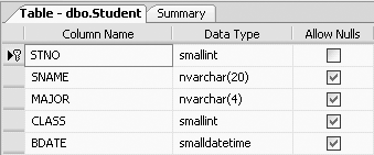
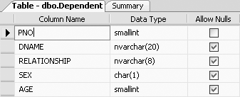
In examining these two tables, we note that student number (stno in the Student table) is the primary key of the Student table. stno is the unique identifier for each student. The Dependent table, which was not created with a primary key of its own, contains a reference to the Student table in that for each dependent, a parent number (pno) is recorded. pno in the Dependent table is a foreign key—it represents a primary key from the table it is referencing, Student. pno in the Dependent table is not unique, because a student can have more than one dependent; that is, one stno can be linked to more than one pno.
From the table descriptions, we can see that the Student table (which has columns stno, sname, major, class, and bdate) can be joined with the Dependent table (which has columns pno, dname, relationship, sex, and age) by columns stno from the Student table and pno from the Dependent table. Following the ANSI JOIN syntax, we can join the two tables as follows:
SELECT stno, sname, relationship, age
FROM Student s JOIN Dependent d
ON s.stno=d.pno
In this construction, Student refers to the Student table and s is the table alias of the Student table. Likewise, Dependent refers to the Dependent table and d is the table alias of the Dependent table. The table alias simplifies writing queries or expressions using single-letter table aliases. We very strongly recommend using table aliases in all multi-table queries. This query requests the student number (stno) and student name (sname) from the Student table, and the relationship and age from the Dependent table when the student number in the Student table (stno) matches a parent number (pno) in the Dependent table.
Tip
Table aliases were discussed in Chapter 2.
When the previous query is typed and executed, you will get the following output showing the dependents of the students:
stno   sname                relationship age
------ -------------------- ------------ ------
2      Lineas               Son          8
2      Lineas               Daughter     9
2      Lineas               Spouse       31
10     Richard              Son          3
10     Richard              Daughter     5
14     Lujack               Son          1
14     Lujack                            3
17     Elainie              Daughter     4
17     Elainie              Son          1
20     Donald               Son          NULL
20     Donald               Son          6
34     Lynette              Daughter     5
34     Lynette              Daughter     1
62     Monica               Husband      45
62     Monica               Son          14
62     Monica               Daughter     16
62     Monica               Daughter     12
123    Holly                Son          5
123    Holly                Son          2
126    Jessica              Son          6
126    Jessica              Son          1
128    Brad                 Son          1
128    Brad                 Daughter     NULL
128    Brad                 Daughter     2
128    Brad                 Wife         26
132    George               Daughter     6
142    Jerry                Daughter     2
143    Cramer               Daughter     7
144    Fraiser              Wife         22
145    Harrison             Wife         22
146    Francis              Wife         22
147    Smithly              Wife         23
147    Smithly              Son          4
147    Smithly              Son          2
147    Smithly              Son          NULL
153    Genevieve            Daughter     5
153    Genevieve            Daughter     4
153    Genevieve            Son          2
158    Thornton             wife         22

 (39 row(s) affected)
To find the course names and the prerequisites of all the courses that have prerequisites, we need to join the Prereq table with the Course table. Course names are in the Course table and the Prereq (prerequisites) table contains the relationship of each course to its prerequisite course. The descriptions of the Prereq table and Course tables are shown in Figures 4-3 and 4-4, respectively.
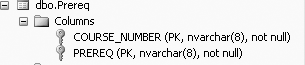
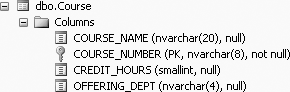
From these descriptions, we first note that the Course table has course_number as its primary key—the unique identifier for each course. The Prereq table also contains a course number, but the course number in the Prereq table is not unique—there are often several prerequisites for any given course. The course number in the Prereq table is a foreign key referencing the primary key of the Course table. The Prereq table (which has columns course_number and prereq) can be joined with the Course table (which has columns course_name, course_number, credit_hours, and offering_dept) by the relationship column in both tables, course_number, as follows:
SELECT *
FROM Course c JOIN Prereq p
ON c.course_number=p.course_number
The same query could be written without the table alias (using a table qualifier) as follows:
SELECT *
FROM Course JOIN Prereq
ON Course.course_number=Prereq.course_number
However, the use of the table alias is so common that the table-alias form should be used. Also, aliases let you select columns that have the same names from the tables. This query will display those rows (12 rows) that have course_number in the Course table equal to course_number in the Prereq table, as follows:
COURSE_NAME          COURSE_NUMBER CREDIT_HOURS OFFERING_DEPT COURSE_NUMBER PREREQ
-------------------- ------------- ------------ ------------- ------------- --------
MANAGERIAL FINANCE   ACCT3333      3            ACCT          ACCT3333     ACCT2220
ORGANIC CHEMISTRY    CHEM3001      3            CHEM          CHEM3001     CHEM2001
DATA STRUCTURES      COSC3320      4            COSC          COSC3320     COSC1310
DATABASE             COSC3380      3            COSC          COSC3380     COSC3320
DATABASE             COSC3380      3            COSC          COSC3380     MATH2410
ADA - INTRODUCTION   COSC5234      4            COSC          COSC5234     COSC3320
ENGLISH COMP II      ENGL1011      3            ENGL          ENGL1011     ENGL1010
FUND. TECH. WRITING  ENGL3401      3            ENGL          ENGL3401     ENGL1011
WRITING FOR NON MAJO ENGL3520      2            ENGL          ENGL3520     ENGL1011
MATH ANALYSIS        MATH5501      3            MATH          MATH5501     MATH2333
AMERICAN GOVERNMENT  POLY2103      2            POLY          POLY2103     POLY1201
POLITICS OF CUBA     POLY5501      4            POLY          POLY5501     POLY4103

 (12 row(s) affected)
Rows from the Course table without a matching row in the Prereq table are not included from the JOIN result set. Courses that do not have prerequisites are not in the result set.
Tip
A primary key is a column or a minimal set of columns whose values uniquely identify a row in a table. A primary key cannot have a null value. Creation of primary keys is discussed in Chapter 11.
The inner join uses equality in the ON clause (the join condition). When an equal sign is used as a join condition, the join is called an equi-join. The use of equi-joins is so common that many people use the phrase “join” synonymously with “equi-join”; when the term “join” is used without qualification, “equi-join” is inferred.
When dealing with table combinations, specifically joins, it is a good idea to estimate the number of rows one might expect in the result set. To find out how many rows will actually occur in the result set, the COUNT function is used. For example:
SELECT COUNT(*)
FROM Course c JOIN Prereq p
ON c.course_number=p.course_number
will tell us that there are 12 rows in the result set.
In any equi join, let us suppose that the two tables to be joined have X number of rows and Y number of rows respectively. How many rows does one expect in the join? A good guideline is in the order of MAX(X,Y). In our case, we have 12 rows in the Prereq table and 32 rows in the Course table. MAX(12,32) = 32, but we actually got 12 rows. MAX(X,Y) is just a guideline. The actual and expected number of rows need not match exactly. It is possible that some Course-Prereq combinations might be repeated.
In SQL Server, the keyword combination INNER JOIN behaves just like the JOIN discussed in the previous section. The general syntax for the INNER JOIN is:
SELECT columns
FROM table1 INNER JOIN table2
ON table1.column1=table2.column1
Using the INNER JOIN, the JOIN query presented in the previous section also could be written as:
SELECT *
FROM Course INNER JOIN Prereq
ON Course.course_number=Prereq.course_number
And, this query too, would produce the same results as given in the previous section.
Another way of joining tables in SQL Server is to use a WHERE clause instead of using the JOIN or INNER JOIN command. According to the SQL-92 standard, the inner join can be specified either with the JOIN/INNER JOIN construction or with a WHERE clause. To perform a join with a WHERE clause, the tables to be joined are listed in the FROM clause of a SELECT statement, and the “join condition” between the tables to be joined is specified in the WHERE clause.
The JOIN from the preceding section could be written with a WHERE clause as follows:
SELECT *
FROM Course c, Prereq p
WHERE c.course_number= p.course_number
This command will display the same 12 rows as was previously shown (when the JOIN was used). You will soon see one of the reasons it is better not to use WHERE.
When two tables are being joined, it does not matter whether TableA is joined with TableB, or TableB is joined with TableA. For example, the following two queries would essentially give the same result set (output):
SELECT *
FROM Course c JOIN Prereq p
ON c.course_number=p.course_number
and:
SELECT *
FROM Prereq p JOIN Course c
ON p.course_number=c.course_number
The only difference in the two result sets would be the order of the columns
. But the result set column order can be controlled by listing out the columns in the order that you want them after the SELECT instead of using the SELECT * syntax.
Joins have to be performed on “compatible” columns; that is, a character column may be joined to another character column, a numeric column may be joined to another numeric column, and so forth. So, for example, a CHAR column can be joined to a VARCHAR column (both being character columns), or an INT column can be joined to a REAL column (both being numeric columns). Having made the point that compatible columns are required, and keeping in mind that SQL is not logical, it is up to the programmer to match semantics. In reality, why would you join two tables unless a relationship existed? If you ask SQL to join a job_title column with a last_name column, it will try to do so even though it makes no sense!
Some columns types--for example, IMAGE--cannot be joined, as these columns will generally not contain “like” columns. Joins cannot be operated on binary data types.
In a SQL statement, a Cartesian product
is where every row of the first table in the FROM clause is joined with each and every row of the second table in the FROM clause. A Cartesian product is produced when the WHERE form of the JOIN is used without the WHERE. An example of a Cartesian product (join) would be:
SELECT *
FROM Course c, Prereq p
The preceding command combines all the data in both the tables and makes a new result set. All rows in the Course table are matched with all rows in the Prereq table (a Cartesian product). This produces 384 rows of output, of which we show the first 10 rows here:
COURSE_NAME          COURSE_NUMBER CREDIT_HOURS OFFERING_DEPT COURSE_NUMBER PREREQ
-------------------- ------------- ------------ ------------- ------------- -------
ACCOUNTING I         ACCT2020      3            ACCT          ACCT3333     ACCT2220
ACCOUNTING II        ACCT2220      3            ACCT          ACCT3333     ACCT2220
MANAGERIAL FINANCE   ACCT3333      3            ACCT          ACCT3333     ACCT2220
ACCOUNTING INFO SYST ACCT3464      3            ACCT          ACCT3333     ACCT2220
INTRO TO CHEMISTRY   CHEM2001      3            CHEM          ACCT3333     ACCT2220
ORGANIC CHEMISTRY    CHEM3001      3            CHEM          ACCT3333     ACCT2220
INTRO TO COMPUTER SC COSC1310      4            COSC          ACCT3333     ACCT2220
TURBO PASCAL         COSC2025      3            COSC          ACCT3333     ACCT2220
ADVANCED COBOL       COSC2303      3            COSC          ACCT3333     ACCT2220
DATA STRUCTURES      COSC3320      4            COSC          ACCT3333     ACCT2220
.
.
.
 (384 row(s) affected)
As we pointed out earlier, before combining tables, it is a good idea to get a count of the number of rows one might expect. This can be done by:
SELECT COUNT(*) AS [COUNT OF CARTESIAN]
FROM Course c, Prereq p
which produces the following output:
COUNT OF CARTESIAN
------------------
384

(1 row(s) affected)
From these results, we can see that the results of a Cartesian “join” will be a relation, say Q, which will have n*m rows (where n is the number of rows from the first relation, and m is the number of rows from the second relation). In the preceding example, the result set has 384 rows (32 times 12), with all possible combinations of rows from the Course table and the Prereq table. If we compare these results with the results of the earlier query (with the WHERE clause), we can see that both the results have the same structure, but the earlier one has been row-filtered by the WHERE clause to include only those rows where there is equality between Course.course_number and Prereq.course_number. Put another way, the earlier results make more sense because they present only those rows that correspond to one another. In this example, the Cartesian product produces extra, meaningless rows.
Oftentimes, the Cartesian product is the result of a user having forgotten to use an appropriate WHERE clause in the SELECT statement when formulating a join using the WHERE format. Note that if the JOIN or INNER JOIN syntax (ANSI JOIN syntax) is used, one cannot avoid the ON clause (no ON clause produces a syntax error). Hence, producing a Cartesian product inadvertently in SQL Server 2005 using the JOIN/INNER JOIN is much harder to do.
Though the Cartesian product is generally regarded as not so useful in SQL per se, if harnessed properly, a Cartesian product can be used to produce exceptionally useful result sets, for example:
The Cartesian product can be used to generate sample or test data.
The simplest Cartesian product of two sets is a two-dimensional table or a cross-tabulation whose cells may be used to enter frequencies or to designate possibilities.
The Cartesian product is needed if you want a collection of all ordered n-tuples (rows with n columns) that can be formed so that they contain one element of the first set, one element of the second set, . . ., and one element of the nth set. For example, if set (or table) X is the 13-element set { A, K, Q, J, 10, 9, 8, 7, 6, 5, 4, 3, 2} and set (or table) Y is the 4-element set {spades, hearts, diamonds, clubs}, then the Cartesian product of those two sets is the 52-element set { (A, spades), (K, spades), . . ., (2, spades), (A, hearts), . . ., (3, clubs), (2, clubs) }.
In SQL Server, a CROSS JOIN can be used to return a Cartesian product of two tables. The form of the CROSS JOIN is:
SELECT *
FROM Table1 CROSS JOIN Table2
Using our database, Student_course, the following CROSS JOIN would produce the same result (Cartesian product) as the query (without the WHERE clause) used in the earlier section:
SELECT *
FROM Course CROSS JOIN Prereq p
Joins with comparison (non-equal) operators—that is, =, >, >=, <, <=, and <>--on the WHERE or ON clauses are called theta joins, where theta represents the relational operator. Inner joins with an = operator are called equi-joins
and joins with an operator other than an = sign are called non-equi-joins
.
The most common join involves join conditions with equality comparisons. Such a join, where the comparison operator is = in the WHERE or ON clause, is called an equi-join. The following is an example:
SELECT *
FROM Course c JOIN Prereq p
ON c.course_number=p.course_number
Another way to look at a join of any kind is that it is the Cartesian product with an added condition. The output for this query has been shown earlier in this chapter. You will note that the result of the join is simply the Cartesian product with the rows where the course numbers are equal. Per the output, you will see that this query displays all rows that have course_number in the Course table equal to course_number in the Prereq table. All the join columns have been included in this result set. This means that course_number has been shown twice—once from the Course table, and once from the Prereq table—and, this duplicate column is of course redundant.
On some occasions, you will need to join a table with itself. Joining a table with itself is known as a self join.
In a regular join, a row of a table (Table A) is joined with a row of another table (Table B) if the column value used for the join in Table A matches the column value used for the join in Table B. One row of a table is processed at a time. But, if the information that you need is contained in several different rows of the same table, for example if you need to compare row1, column1, with row2, column1, you will need to join the table with itself.
Suppose that we want to find all the students who are more senior than other students. We have to join the Student table with itself. Logically, we need to take a row from the Student table and look through the rest of the Student table to see which rows fit the criterion (“more senior”). To accomplish this, we will use two versions of the Student table. Here is our query:
SELECT 'SENIORITY' = x.sname + ' is in a higher class than ' + y.sname
FROM Student AS x, Student AS y
WHERE y.class = 3
AND x.class > y.class
First we alias the Student table as x, and then we alias another instance of the Student table as y. Then we join where x.class is greater than y.class and we added the WHERE qualifier y.class = 3, so this effectively gives us only the seniors. We restricted the result to “just seniors” to keep the result set smaller). The use of the > sign is also an example of a non-equi-join.
Tip
+ is a string concatenation operator in SQL Server. String concatenation is discussed in detail in the next chapter.
This query produces the 70 rows of output (of which we show a sample):
SENIORITY
-------------------------------------------------------------
Mary is in a higher class than Susan
Kelly is in a higher class than Susan
Donald is in a higher class than Susan
Chris is in a higher class than Susan
Jake is in a higher class than Susan
Holly is in a higher class than Susan
Jerry is in a higher class than Susan
Harrison is in a higher class than Susan
Francis is in a higher class than Susan
Benny is in a higher class than Susan
Mary is in a higher class than Monica
Kelly is in a higher class than Monica
Donald is in a higher class than Monica
.
.
.
Mary is in a higher class than Phoebe
Kelly is in a higher class than Phoebe
Donald is in a higher class than Phoebe
.
.
.
Mary is in a higher class than Rachel
Kelly is in a higher class than Rachel
Donald is in a higher class than Rachel
.
.
.
Mary is in a higher class than Cramer
Kelly is in a higher class than Cramer
Donald is in a higher class than Cramer
.
.
.
(70 row(s) affected)
In this join, all the rows where x.class is greater than y.class (which is restricted to 3) are joined to the rows that have y.class = 3. So Mary, the first row that has x.class = 4, is joined to the first row where class = 3 (y.class = 3), which is Susan. Then, the next row in the Student table with x.class = 4 is Kelly, so Kelly is joined to Susan (y.class = 3), etc.
The alternative INNER JOIN syntax for this non-equi-join is:
SELECT 'SENIORITY' = x.sname + ' is more senior than ' + y.sname
FROM Student AS x INNER JOIN Student AS y
ON x.class > y.class
WHERE y.class = 3
As with other SELECT statements, the ORDER BY clause can be used in joins to order the result set. For example, to order the result set (output) of one of the queries presented earlier in this chapter by the course_number column, we would type the following:
SELECT c.course_name, c.course_number, c.credit_hours, c.offering_dept, p.prereq
FROM Course c JOIN Prereq p
ON c.course_number=p.course_number
ORDER BY c.course_number
Or this alternative:
SELECT c.course_name, c.course_number, c.credit_hours, c.offering_dept, p.prereq
FROM Course c JOIN Prereq p
ON c.course_number=p.course_number
ORDER BY 2
ORDER BY 2 means to order by the second column of the result set. This query produces the same 12 rows as the previous query, but ordered alphabetically in the order of course_number:
COURSE_NAME          COURSE_NUMBER CREDIT_HOURS OFFERING_DEPT PREREQ
-------------------- ------------- ------------ ------------- --------
MANAGERIAL FINANCE   ACCT3333      3         ACCT          ACCT2220
ORGANIC CHEMISTRY    CHEM3001      3         CHEM          CHEM2001
DATA STRUCTURES      COSC3320      4         COSC          COSC1310
DATABASE             COSC3380      3         COSC          COSC3320
DATABASE             COSC3380      3         COSC          MATH2410
ADA - INTRODUCTION   COSC5234      4         COSC          COSC3320
ENGLISH COMP II      ENGL1011      3         ENGL          ENGL1010
FUND. TECH. WRITING  ENGL3401      3         ENGL          ENGL1011
WRITING FOR NON MAJO ENGL3520      2         ENGL          ENGL1011
MATH ANALYSIS        MATH5501      3         MATH          MATH2333
AMERICAN GOVERNMENT  POLY2103      2         POLY          POLY1201
POLITICS OF CUBA     POLY5501      4         POLY          POLY4103

(12 row(s) affected)
You will frequently need to perform a join in which you have to get data from more than two tables. A join is a pair-wise, binary operation. In SQL Server, you can join more than two tables in either of two ways: by using a nested JOIN, or by using a WHERE clause. Joins are always done pair-wise.
The simplest form of the nested JOIN is as follows:
SELECT columns
FROM table1 JOIN
(table2 JOIN table3
ON table3.column3=table2.column2)
ON table1.column1=table2.column2
Here Tables 2 and 3 are joined to form a virtual table that is then joined to Table 1 to create your result set. Note that the join in parentheses is completed first.
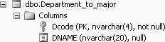
As an example of a nested join, if we want to see the courses (course names and numbers) that have prerequisites and the departments (department names) offering those courses, we will have to join three tables--Course, Prereq, and Department_to_major, because the data that we want to display is spread among these three tables. We could choose to first join the Course table with the Prereq table, and then join that result to the Department_to_major table. The Department_to_major table contains the names of the departments. To determine which columns of the Department_to_major table can be used in the join, we have to also look at the description of the Department_to_major table, which is shown in Figure 4-5.
The query to join the Course table to the Prereq table to the Department_to_major table with the Course/Prereq join done first is:
SELECT c.course_name, c.course_number, d2m.dname
FROM department_to_major d2m JOIN
(course c JOIN prereq  p
ON c.course_number=p.course_number)
ON c.offering_dept=d2m.dcode
In the nested JOIN, the part within the parentheses, course c JOIN prereq p ON c.course_number=p.course_number, is performed first to produce a result set. The internal result is then used to join to the third table, Department_to_major.
The result of the join is the following 12 rows:
course_name          course_number dname
-------------------- ------------- --------------------
MANAGERIAL FINANCE   ACCT3333      Accounting
ORGANIC CHEMISTRY    CHEM3001      Chemistry
DATA STRUCTURES      COSC3320      Computer Science
DATABASE             COSC3380      Computer Science
DATABASE             COSC3380      Computer Science
ADA - INTRODUCTION   COSC5234      Computer Science
ENGLISH COMP II      ENGL1011      English
FUND. TECH. WRITING  ENGL3401      English
WRITING FOR NON MAJO ENGL3520      English
Math Analysis        MATH5501      Mathematics
AMERICAN GOVERNMENT  POLY2103      Political Science
POLITICS OF CUBA     POLY5501      Political Science

 (12 row(s) affected)
Which join is performed first has performance implications. We could choose to do the Course/Department_to_major table join first, in which case the query could be written as follows:
SELECT c.course_name, c.course_number, d.dname
FROM (course c JOIN department_to_major d
ON c.offering_dept = d.dcode)
JOIN prereq p
ON p.course_number = c.course_number
For larger tables and multi-table joins, the order will determine which version of the query would be most efficient.
In an equi-inner join, rows without matching values are eliminated from the join result. For example, with the following join, we did not see information on any course that did not have a prerequisite:
SELECT *
FROM Course c, Prereq p
WHERE c.course_number = p.course_number
In some cases, it may be desirable to include rows from one table even if it does not have matching rows in the other table. This is done by the use of an OUTER JOIN. OUTER JOINs are used when we want to keep all the rows from the one table, such as Course, or all the rows from the other, regardless of whether they have matching rows in the other table. In SQL Server, an OUTER JOIN in which we want to keep all the rows from the first (left) table is called a LEFT OUTER JOIN,
and an OUTER JOIN in which we want to keep all the rows from the second table (or right relation) is called the RIGHT OUTER JOIN. The term FULL OUTER JOIN is used to designate the union of the LEFT and RIGHT OUTER JOINs. In the following subsections, we illustrate the LEFT OUTER JOIN, RIGHT OUTER JOIN, and FULL OUTER JOIN.
LEFT OUTER JOINs include all the rows from the first (left) of the two tables, even if there are no matching values for the rows in the second (right) table. LEFT OUTER JOINs are performed in SQL Server using a LEFT OUTER JOIN statement.
Tip
LEFT JOIN is the same as LEFT OUTER JOIN. The inclusion of the word OUTER is optional in SQL Server SQL, but we will use LEFT OUTER JOIN instead of LEFT JOIN for clarity.
The following is the simplest form of a LEFT OUTER JOIN statement:
SELECT columns
FROM table1 LEFT OUTER JOIN table2
ON table1.column1=table2.column1
For example, if we want to list all the rows in the Course table (the left, or first table), even if these courses do not have prerequisites, we type the following LEFT OUTER JOIN statement:
SELECT *
FROM Course c LEFT OUTER JOIN Prereq p
ON c.course_number = p.course_number
Here the LEFT OUTER JOIN is processed as follows: First, all the rows from the Course table that have course_number equal to the course_number in the Prereq table are joined. Then, when a row (with a course_number) from the Course table (first table) has no match in Prereq table (second table), the rows from the Course table are anyway included in the result set with a row of null values joined to the right side. This means that the courses that do not have prerequisites will get a set of null values for prerequisites. So, the output (result set) of a LEFT OUTER JOIN includes all rows from the left (first) table, which in this case is the Course table with matching Prereq rows where applicable.
Tip
The use of the *= operator for the LEFT OUTER JOIN is considered old syntax, and hence its use is not encouraged. It is prone to ambiguities, especially when joining three or more tables.
The previous query will produce the following 33 rows of output (of which we show the first 13 rows here):
COURSE_NAME          COURSE_NUMBER CREDIT_HOURS OFFERING_DEPT COURSE_NUMBER PREREQ
-------------------- ------------- ------------ ------------- ------------- -------
ACCOUNTING I         ACCT2020      3            ACCT          NULL          NULL
ACCOUNTING II        ACCT2220      3            ACCT          NULL          NULL
MANAGERIAL FINANCE   ACCT3333      3            ACCT          ACCT3333     ACCT2220
ACCOUNTING INFO SYST ACCT3464      3            ACCT          NULL          NULL
INTRO TO CHEMISTRY   CHEM2001      3            CHEM          NULL          NULL
ORGANIC CHEMISTRY    CHEM3001      3            CHEM          CHEM3001     CHEM2001
INTRO TO COMPUTER SC COSC1310      4            COSC          NULL          NULL
TURBO PASCAL         COSC2025      3            COSC          NULL          NULL
ADVANCED COBOL       COSC2303      3            COSC          NULL          NULL
DATA STRUCTURES      COSC3320      4            COSC          COSC3320     COSC1310
DATABASE             COSC3380      3            COSC          COSC3380     COSC3320
DATABASE             COSC3380      3            COSC          COSC3380     MATH2410
OPERATIONS RESEARCH  COSC3701      3            COSC          NULL          NULL
.
.
.

(33 row(s) affected)
Note the nulls added to courses (due to the LEFT OUTER JOIN) like ACCOUNTING I, ACCOUNTING II, ACCOUNTING INFO SYST, and so on, which are the courses (in the Course table) that do not have prerequisites.
RIGHT OUTER JOINs include all the rows from the second (right) of the two tables, even if there are no matching values for the rows in the first (left) table. RIGHT OUTER JOINs are performed in SQL Server using a RIGHT OUTER JOIN statement.
Tip
RIGHT JOIN is the same as RIGHT OUTER JOIN. The inclusion of the word OUTER is optional in SQL Server SQL, but we will use RIGHT OUTER JOIN instead of RIGHT JOIN for clarity’s sake.
The following is the simplest form of a RIGHT OUTER JOIN statement:
SELECT columns
FROM table1 RIGHT OUTER JOIN table2
ON table1.fieldcolumn1=table2.column1
As an example, we will redo the previous query from the right side. If we want to list all the rows in the Course table (the right, or second table), even if these courses do not have prerequisites, we may type the following RIGHT OUTER JOIN statement:
SELECT *
FROM Prereq p RIGHT OUTER JOIN Course c
ON p.course_number = c.course_number
Here, the RIGHT OUTER JOIN is processed as follows. First, all the rows from the Prereq table that have course_number equal to the course_number in the Course table are joined. Then, when a row (with a course_number) from the Course table (second table) has no match in the Prereq table (first table), the rows from the Course table are anyway included in the result set with a row of null values joined to the left side. This means that courses that do not have prerequisites will get a set of null values joined to the left side. The output of a RIGHT OUTER JOIN includes all rows from the right (second) table, which in this case is the Course table, producing output similar to that obtained in the previous section.
The output consists of 33 rows (of which the first 13 rows are shown here):
COURSE_NUMBER PREREQ   COURSE_NAME         COURSE_NUMBER CREDIT_HOURS OFFERING_DEPT
------------- -------- -------------------- ------------- ------------ ------------
NULL          NULL     ACCOUNTING I         ACCT2020      3            ACCT
NULL          NULL     ACCOUNTING II        ACCT2220      3            ACCT
ACCT3333      ACCT2220 MANAGERIAL FINANCE   ACCT3333      3            ACCT
NULL          NULL     ACCOUNTING INFO SYST ACCT3464      3            ACCT
NULL          NULL     INTRO TO CHEMISTRY   CHEM2001      3            CHEM
CHEM3001      CHEM2001 ORGANIC CHEMISTRY    CHEM3001      3            CHEM
NULL          NULL     INTRO TO COMPUTER SC COSC1310      4            COSC
NULL          NULL     TURBO PASCAL         COSC2025      3            COSC
NULL          NULL     ADVANCED COBOL       COSC2303      3            COSC
COSC3320      COSC1310 DATA STRUCTURES      COSC3320      4            COSC
COSC3380      COSC3320 DATABASE             COSC3380      3            COSC
COSC3380      MATH2410 DATABASE             COSC3380      3            COSC
NULL          NULL     OPERATIONS RESEARCH  COSC3701      3            COSC
.
.
.

(33 row(s) affected)
Once again, note the NULLs added to the unmatched rows from the second table due to the use of the RIGHT OUTER JOIN.
The FULL OUTER JOIN includes the rows that are equi-joined from both tables, plus the remaining rows from the first table and the remaining rows from the second table. NULLs are added to the unmatched rows from both the first and second tables.
The following is the simplest form of a FULL OUTER JOIN statement:
SELECT columns
FROM table1 FULL OUTER JOIN table2
ON table1.column1=table2.column1
If we want to list all the rows for which a connection exists between the Prereq table and the Course table (result of a regular JOIN), and in addition, we want all rows from the Prereq table for which there is no corresponding row in the Course table (LEFT
OUTER JOIN), and in addition, we want all rows in the Course table for which there is no corresponding row in the Prereq table (RIGHT OUTER JOIN), we would use the following FULL OUTER JOIN statement:
SELECT *
FROM Prereq p FULL OUTER JOIN Course c
ON p.course_number = c.course_number
We will get 33 rows:
COURSE_NUMBER PREREQ   COURSE_NAME         COURSE_NUMBER CREDIT_HOURS OFFERING_DEPT
------------- -------- -------------------- ------------- ------------ ------------
NULL          NULL     ACCOUNTING I         ACCT2020      3            ACCT
NULL          NULL     ACCOUNTING II        ACCT2220      3            ACCT
ACCT3333      ACCT2220 MANAGERIAL FINANCE   ACCT3333      3            ACCT
NULL          NULL     ACCOUNTING INFO SYST ACCT3464      3            ACCT
NULL          NULL     INTRO TO CHEMISTRY   CHEM2001      3            CHEM
CHEM3001      CHEM2001 ORGANIC CHEMISTRY    CHEM3001      3            CHEM
NULL          NULL     INTRO TO COMPUTER SC COSC1310      4            COSC
NULL          NULL     TURBO PASCAL         COSC2025      3            COSC
NULL          NULL     ADVANCED COBOL       COSC2303      3            COSC
COSC3320      COSC1310 DATA STRUCTURES      COSC3320      4            COSC
COSC3380      COSC3320 DATABASE             COSC3380      3            COSC
COSC3380      MATH2410 DATABASE             COSC3380      3            COSC
NULL          NULL     OPERATIONS RESEARCH  COSC3701      3            COSC
NULL          NULL     ADVANCED ASSEMBLER   COSC4301      3            COSC
NULL          NULL     SYSTEM PROJECT       COSC4309      3            COSC
COSC5234      COSC3320 ADA - INTRODUCTION   COSC5234      4            COSC
NULL          NULL     NETWORKS             COSC5920      3            COSC
NULL          NULL     ENGLISH COMP I       ENGL1010      3            ENGL
ENGL1011      ENGL1010 ENGLISH COMP II      ENGL1011      3            ENGL
ENGL3401      ENGL1011 FUND. TECH. WRITING  ENGL3401      3            ENGL
NULL          NULL     TECHNICAL WRITING    ENGL3402      2            ENGL
ENGL3520      ENGL1011 WRITING FOR NON MAJO ENGL3520      2            ENGL
NULL          NULL     CALCULUS 1           MATH1501      4            MATH
NULL          NULL     CALCULUS 2           MATH1502      3            MATH
NULL          NULL     CALCULUS 3           MATH1503      3            MATH
NULL          NULL     ALGEBRA              MATH2333      3            MATH
NULL          NULL     DISCRETE MATHEMATICS MATH2410      3            MATH
MATH5501      MATH2333 Math Analysis        MATH5501      3            MATH
NULL          NULL     AMERICAN CONSTITUTIO POLY1201      1            POLY
NULL          NULL     INTRO TO POLITICAL S POLY2001      3            POLY
POLY2103      POLY1201 AMERICAN GOVERNMENT  POLY2103      2            POLY
NULL          NULL     SOCIALISM AND COMMUN POLY4103      4            POLY
POLY5501      POLY4103 POLITICS OF CUBA     POLY5501      4            POLY

 (33 row(s) affected)
After reading this chapter, you should have an appreciation of the concept of the join, a concept very fundamental to understanding relational databases. We have illustrated, with examples, the regular JOIN, CROSS JOIN and the Cartesian product, equi-joins and non-equi-joins, the self join, LEFT OUTER JOIN, RIGHT OUTER JOIN, and FULL OUTER JOIN. We have also discussed how multiple tables can be joined using a nested join.
What is a join? Why do you need a join?
What is an
INNER JOIN?Which clause[s] can be used in place of the
JOINin Server SQL?What is the Cartesian product?
What would be the Cartesian product of a table with 15 rows and another table with 23 rows?
List some uses of the Cartesian product.
What is an equi-join?
What is a non-equi-join? Give an example of an non-equi-join.
What is a self join? Give an example of a self join.
What is a
LEFT OUTER JOIN?What is a
RIGHT OUTER JOIN?What is a
CROSS JOIN?What is a
FULL OUTER JOIN?Does Server SQL allow the use of
*=to perform outer joins?What is the maximum number of rows that a self join can produce?
For what kinds of joins will the associative property hold?
What would be the Cartesian product of the two sets {a,b,c} and {c,d,e}?
Unless specified otherwise, use the Student_course database to answer the following questions. Also, use appropriate column headings when displaying your output.
Create two tables,
Stu(name,majorCode) andMajor(majorCode,majorDesc), with the following data. UseVARCHARfor the codes and appropriate data types for the other columns.StunamemajorCodeJonesCSSmithACEvansMAAdamsCSSumonMajormajorCodemajorDescACAccountingCSComputer ScienceMAMathHIHistoryDisplay the Cartesian product (no
WHEREclause) of the two tables. UseSELECT *.... How many rows did you get? How many rows will you always get when combining two tables with n and m rows in them (Cartesian product)?Display an equi-join of the
StuandMajortables onmajorCode. First do this using theINNER JOIN, and then display the results using the equi-join with an appropriateWHEREclause. Use appropriate table aliases. How many rows did you get?Display whatever you get if you leave off the column qualifiers (the aliases) on the equi-join in question 1b. (Note: This will give an error because of ambiguous column names.)
Use the
COUNT(*)function instead ofSELECT *in the query. UseCOUNTto show the number of rows in the result set of the equi-join.Display the
name,majorCode, andmajorDescof all students regardless of whether or not they have a declared major (even if the major column is null). (Hint: You need to use aLEFT OUTER JOINhere ifStuis the first table in your equi-join query.)Display a list of
majorDescsavailable (even if themajorDescdoes not have students yet) and the students in each of the majors. (Hint: You need to use aRIGHT OUTER JOINhere.)Display the Cartesian product of the two tables using a
CROSS JOIN.
Create two tables,
T1(name,jobno) andT2(jobno,jobdesc). Letjobnobe data typeINT, and use appropriate data types for the other columns. Put three rows inT1and two rows inT2. GiveT1.jobnovalues 1, 2, 3 for the three rows: <..., 1>,<..., 2,>,<..., 3>, where...represents any value you choose. GiveT2.jobnothe values 1, 2: <1,...>,<2,...>.How many rows are in the equi-join (on
jobno) ofT1andT2?If the values of
T2.jobnowere <2,...>, <2,...> (with differentjobdescvalues), how many rows would you expect to get, and why? Why would the rows have to have different descriptions?If the values of
T2.jobnowere 4, 5 as in <4,...>,<5,...>, how many rows would you expect to get?If the values of
T1.jobnowere <..., 1>,<..., 1>,<..., 1> (with different names) and the values ofT2.jobnowere <1,...>,<1...> with different descriptions, how many rows would you expect to get?If you have two tables, what is the number of rows you may expect from an equi-join operation (and with what conditions)? A Cartesian product?
The number of rows in an equi-join of two tables, whose sizes are m and n rows, is from ___ to ____ depending on these conditions: _________ .
Use tables
T1andT2in this exercise. Create another table calledT3(jobdesc,minpay). Letminpaybe of data typeSMALLMONEY. Populate the table with at least one occurrence of eachjobdescfrom tableT2plus one morejobdescthat is not inT2. Write and display the result of a triple equi-join ofT1,T2, andT3. Use an appropriate comment on each of the lines of theWHEREclause on which there are equi-join conditions. (Note: You will need two equi-join conditions.)How many rows did you get in the equi-join?
Use the
COUNT(*)function and display the number of rows in the equi-join.How many rows would you get in this meaningless, triple Cartesian product (use
COUNT(*))?In an equi-join of n tables, you always have _______ _ equi-join conditions in the
WHEREclause.In the preceding three exercises, you created tables
T1,T2,T3,Stu, andMajor. When you have completed the three exercises, delete these tables.Answer questions 4 through 8 by using the
Student_coursedatabase.
Display a list of course names for all of the prerequisite courses.
Use a
JOINorINNER JOINto join theSectionandCoursetables.List the course names, instructors, the semesters and years they were teaching in.
List the instructor, course names, and offering departments of each of the courses the instructors were teaching.
Use a
LEFT OUTER JOINto join theSectionandCoursetables.List the course names, instructors, and the semesters and years they were teaching in. Sort in descending order by instructors.
List the instructor, course names, and offering departments of each of the courses the instructors were teaching.
Use a
RIGHT OUTER JOINto join theSectionandCoursetables.For each instructor, list the name of each course they teach and the semester and year in which they teach that course.
For each course, list the name of the instructor and the name of the department in which it is offered.
Are there any differences in the answers for questions 5, 6, and 7? Why? Explain.
Use a
FULL OUTER JOINto join theSectionandCoursetables. How do the results vary from the results of questions 5, 6, and 7?
Discuss the output that the following query would produce:
SELECT *
FROM Course AS c, Prereq AS p
WHERE c.course_number<>p.course_number
Find all the sophomores who are more senior than other students. (Hint: Use a self-join.)
Find all the courses that have more credit hours than other courses. (Hint: Use a self-join.)
Display a list of the names of all students who have dependents, the dependents name, relationship and age, ordered by the age of the dependent.
Get Learning SQL on SQL Server 2005 now with the O’Reilly learning platform.
O’Reilly members experience books, live events, courses curated by job role, and more from O’Reilly and nearly 200 top publishers.

