Loss Models: From Data to Decisions, 4th Edition

9.3 The compound model for aggregate claims

Let S denote aggregate losses associated with a set of N observed claims X₁, X₂, …, X_N satisfying the independence assumptions following (9.1). The approach in this chapter involves the following three steps:

1. Develop a model for the distribution of N based on data.

2. Develop a model for the common distribution of the X_js based on data.

3. Using these two models, carry out necessary calculations to obtain the distribution of S.

Completion of the first two steps follows the ideas developed elsewhere in this text. We now presume that these two models are developed and that we only need to carry out numerical work in obtaining solutions to problems associated with the distribution of S.

The random sum

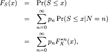
(where N has a counting distribution) has distribution function

(9.3)

where F_X(x) = Pr(X ≤ x) is the common distribution function of the X_js and p_n = Pr(N = n). The distribution of S is called a compound distribution. In (9.3), F_X^*n(x) is the “n-fold convolution” of the cdf of X. It can be obtained as

and

(9.4)

The tail may then be written, ...