Mastering Algorithms with C

Computational Complexity

When speaking of the performance of an algorithm, usually the aspect of interest is its complexity, which is the growth rate of the resources (usually time) it requires with respect to the size of the data it processes. O -notation describes an algorithm’s complexity. Using O -notation, we can frequently describe the worst-case complexity of an algorithm simply by inspecting its overall structure. Other times, it is helpful to employ techniques involving recurrences and summation formulas (see the related topics at the end of the chapter), and statistics.

To understand complexity, let’s look at one way to surmise the resources an algorithm will require. It should seem reasonable that if we look at an algorithm as a series of k statements, each with some cost (usually time) to execute, c_i , we can determine the algorithm’s total cost by summing the costs of all statements from c ₁ to c_k in whatever order each is executed. Normally statements are executed in a more complicated manner than simply in sequence, so this has to be taken into account when totaling the costs. For example, if some subset of the statements is executed in a loop, the costs of the subset must be multiplied by the number of iterations. Consider an algorithm consisting of k = 6 statements. If statements 3, 4, and 5 are executed in a loop from 1 to n and the other statements are executed sequentially, the overall cost of the algorithm is:

T(n) = c ₁ + c ₂ + n(c ₃ + c ₄ + c ₅) + c ₆

Using the rules of O -notation, this algorithm’s complexity is O (n) because the constants are not significant. Analyzing an algorithm in terms of these constant costs is very thorough. However, recalling what we have seen about growth rates, remember that we do not need to be so precise. When inspecting the overall structure of an algorithm, only two steps need to be performed: we must determine which parts of the algorithm depend on data whose size is not constant, and then derive functions that describe the performance of each part. All other parts of the algorithm execute with a constant cost and can be ignored in figuring its overall complexity.

Assuming T (n) in the previous example represents an algorithm’s running time, it is important to realize that O (n), its complexity, says little about the actual time the algorithm will take to run. In other words, just because an algorithm has a low growth rate does not necessarily mean it will execute in a small amount of time. In fact, complexities have no real units of measurement at all. They describe only how the resource being measured will be affected by a change in data size. For example, saying that T (n) is O (n) conveys only that the algorithm’s running time varies proportionally to n, and that n is an upper bound for T (n) within a constant factor. Formally, we say that T (n) ≤ cn, where c is a constant factor that accounts for various costs not associated with the data, such as the type of computer on which the algorithm is running, the compiler used to generate the machine code, and constants in the algorithm itself.

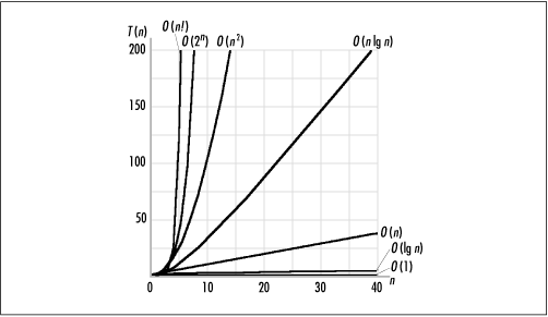
Many complexities occur frequently in computing, so it is worthwhile to become familiar with them. Table 4.1 lists some typical situations in which common complexities occur. Table 4.2 lists these common complexities along with some calculations illustrating their growth rates. Figure 4.1 presents the data of Table 4.2 in a graphical form.

Table 4.1. Some Situations Wherein Common Complexities Occur

Complexity	Example
O(1)	Fetching the first element from a set of data
O(lg n)	Splitting a set of data in half, then splitting the halves in half, etc.
O(n)	Traversing a set of data
O(n lg n)	Splitting a set of data in half repeatedly and traversing each half
O(n 2)	Traversing a set of data once for each member of another set of equal size
O(2 n )	Generating all possible subsets of a set of data
O(n!)	Generating all possible permutations of a set of data

Table 4.2. The Growth Rates of the Complexities in Table 4.1

	n = 1	n = 16	n = 256	n = 4K	n = 64K	n = 1M
O(1)	1.000E+00	1.000E+00	1.000E+00	1.000E+00	1.000E+00	1.000E+00
O (lg n)	0.000E+00	4.000E+00	8.000E+00	1.200E+01	1.600E+01	2.000E+01
O (n)	1.000E+00	1.600E+01	2.560E+02	4.096E+03	6.554E+04	1.049E+06
O (n lg n)	0.000E+00	6.400E+01	2.048E+03	4.915E+04	1.049E+06	2.097E+07
O (n 2)	1.000E+00	2.560E+02	6.554E+04	1.678E+07	4.295E+09	1.100E+12
O (2 n )	2.000E+00	6.554E+04	1.158E+77	—	—	—
O (n!)	1.000E+00	2.092E+13	—	—	—	—

Figure 4.1. A graphical depiction of the growth rates in Tables Table 4.1 and Table 4.2

Just as the complexity of an algorithm says little about its actual running time, it is important to understand that no measure of complexity is necessarily efficient or inefficient. Although complexity is an indication of the efficiency of an algorithm, whether a particular complexity is considered efficient or inefficient depends on the problem. Generally, an efficient algorithm is one in which we know we are doing the best we can do given certain criteria. Typically, an algorithm is said to be efficient if there are no algorithms with lower complexities to solve the same problem and the algorithm does not contain excessive constants. Some problems are intractable, so there are no “efficient” solutions without settling for an approximation. This is true of a special class of problems called NP-complete problems (see the related topics at the end of the chapter).

Although an algorithm’s complexity is an important starting point for determining how well it will perform, often there are other things to consider in practice. For example, when two algorithms are of the same complexity, it may be worthwhile to consider their less significant terms and factors. If the data on which the algorithms’ performances depend is small enough, even an algorithm of greater complexity with small constants may perform better in practice than one that has a lower order of complexity and larger constants. Other factors worth considering are how complicated an algorithm will be to develop and maintain, and how we can make the actual implementation of an algorithm more efficient. An efficient implementation does not always affect an algorithm’s complexity, but it can reduce constant factors, which makes the algorithm run faster in practice.