Mastering Algorithms with C

Description of Polynomial Interpolation

There are many problems that can be described in terms of a function. However, often this function is not known, and we must infer what we can about it from only a small number of points. To do this, we interpolate between the points. For example, in Figure 13.1, the known points along f (x) are x ₀, . . ., x ₈, shown by circular black dots. Interpolation helps us get a good idea of the value of the function at points z ₀, z ₁, and z ₂, shown by white squares. This section presents polynomial interpolation.

Figure 13.1. Interpolation with nine points to find the value of a function at other points

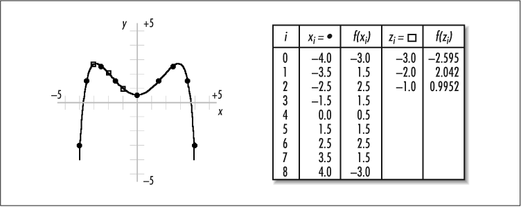
Fundamental to polynomial interpolation is the construction of a special polynomial called an interpolating polynomial. To appreciate the significance of this polynomial, let’s look at some principles of polynomials in general. First, a polynomial is a function of the form:

p(x) = a ₀+a ₁ x+a ₂ x ²+. . . +a _n x ⁿ

where a ₀, . . ., a_n are coefficients. Polynomials of this form are said to have degree n, provided a_n is nonzero. This is the power form of a polynomial, which is especially common in mathematical discussions. However, other forms of polynomials are more convenient in certain contexts. For example, a form particularly relevant to polynomial interpolation is the Newton form:

p(x) = a ₀+a ₁(x-c ₁)+a ₂(x-c ₁)(x-c ₂)+ . . . +a _n(x-c ₁)( ...